ANALYSIS OF VARIANCE ANOVA test of equality of

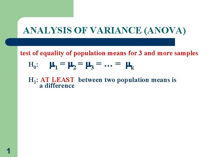
ANALYSIS OF VARIANCE (ANOVA) test of equality of population means for 3 and more samples H 0: 1 = 2 = 3 = … = k H 1: AT LEAST between two population means is a difference 1

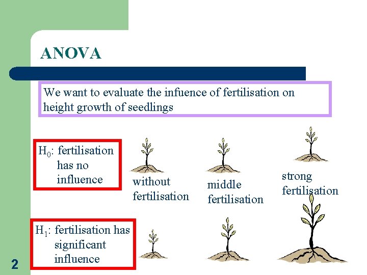
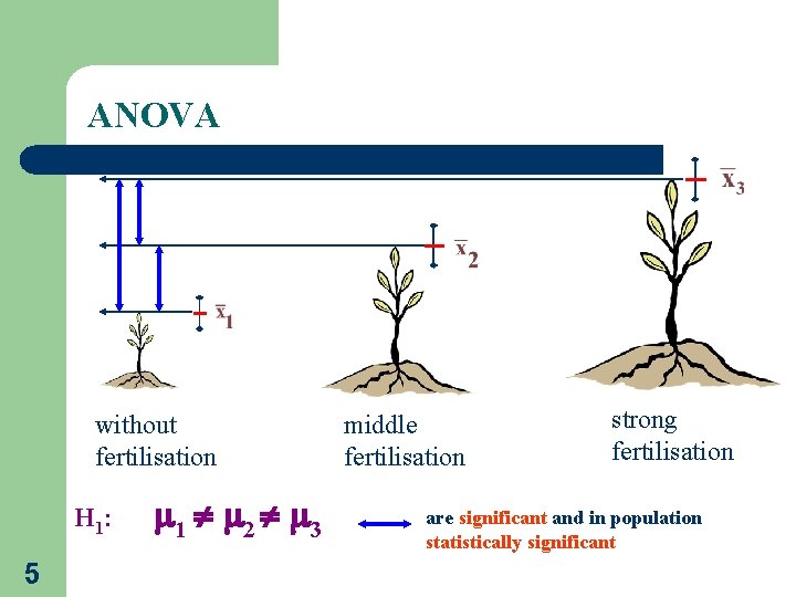
ANOVA We want to evaluate the infuence of fertilisation on height growth of seedlings H 0: fertilisation has no influence 2 H 1: fertilisation has significant influence without fertilisation middle fertilisation strong fertilisation

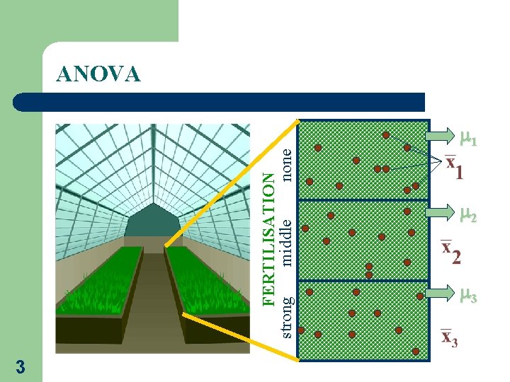
FERTILISATION strong middle none ANOVA 3 1 2 3

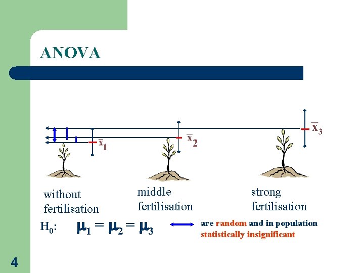
ANOVA without fertilisation H 0: 1 = 4 middle fertilisation 2 = 3 strong fertilisation are random and in population statistically insignificant

ANOVA without fertilisation H 1: 5 1 2 3 middle fertilisation strong fertilisation are significant and in population statistically significant

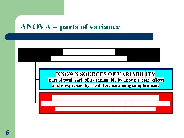
ANOVA – parts of variance 6

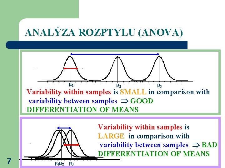
ANALÝZA ROZPTYLU (ANOVA) 1 2 3 Variability within samples is SMALL in comparison with variability between samples GOOD DIFFERENTIATION OF MEANS 7 Variability within samples is LARGE in comparison with variability between samples BAD DIFFERENTIATION OF MEANS 1 2 3

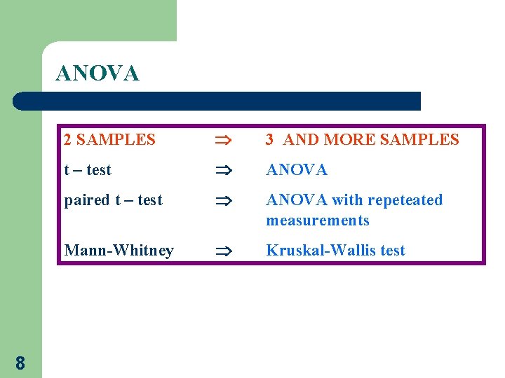
ANOVA 8 2 SAMPLES 3 AND MORE SAMPLES t – test ANOVA paired t – test ANOVA with repeteated measurements Mann-Whitney Kruskal-Wallis test

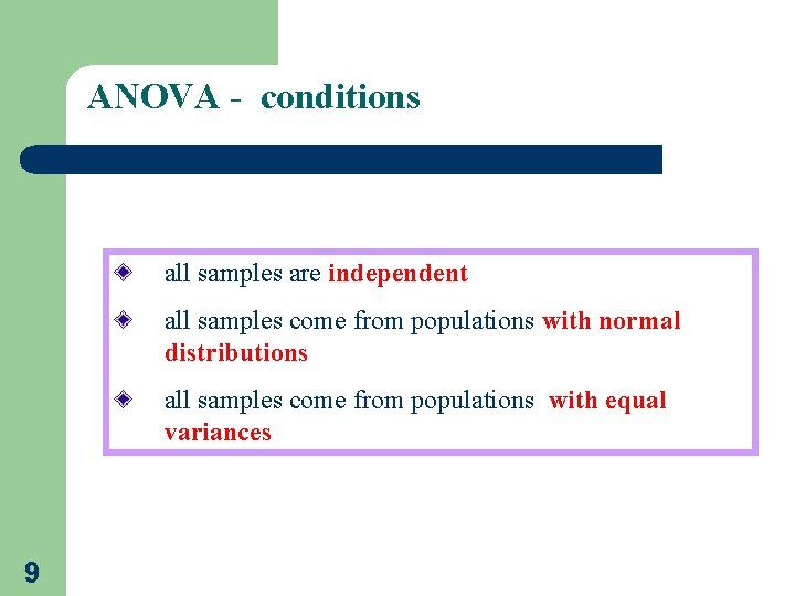
ANOVA - conditions all samples are independent all samples come from populations with normal distributions all samples come from populations with equal variances 9

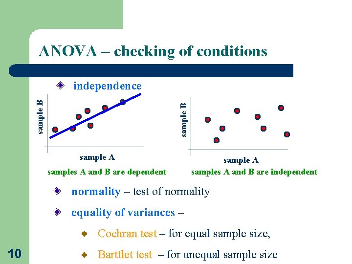
ANOVA – checking of conditions sample B independence sample A samples A and B are dependent sample A samples A and B are independent normality – test of normality equality of variances – Cochran test – for equal sample size, 10 Barttlet test – for unequal sample size

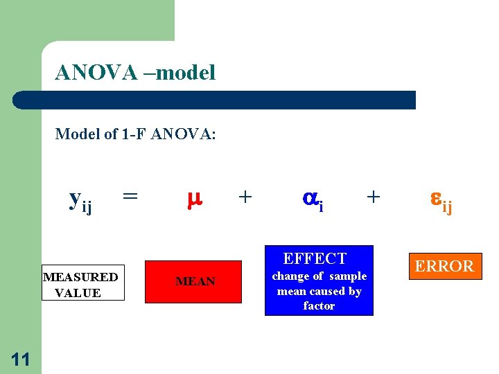
ANOVA –model Model of 1 -F ANOVA: yij = + i EFFECT MEASURED VALUE 11 MEAN change of sample mean caused by factor + ij ERROR

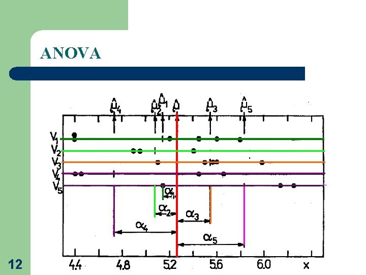
ANOVA 12

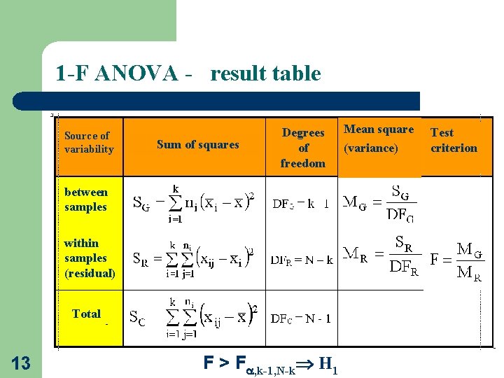
1 -F ANOVA - result table Source of variability Sum of squares Degrees of freedom between samples within samples (residual) Total 13 F > F , k-1, N-k H 1 Mean square (variance) Test criterion

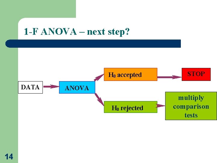
1 -F ANOVA – next step? H 0 accepted DATA ANOVA H 0 rejected 14 STOP multiply comparison tests

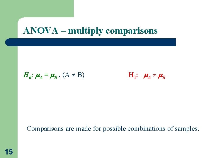
ANOVA – multiply comparisons H 0: A = B , (A B) H 1: A B Comparisons are made for possible combinations of samples. 15

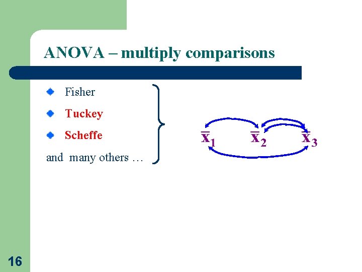
ANOVA – multiply comparisons Fisher Tuckey Scheffe and many others … 16

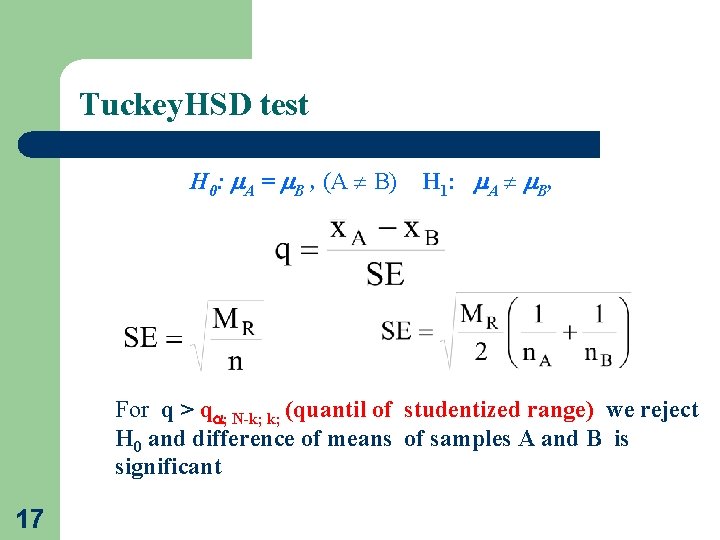
Tuckey. HSD test H 0: A = B , (A B) H 1: A B , For q > q ; N-k; k; (quantil of studentized range) we reject H 0 and difference of means of samples A and B is significant 17

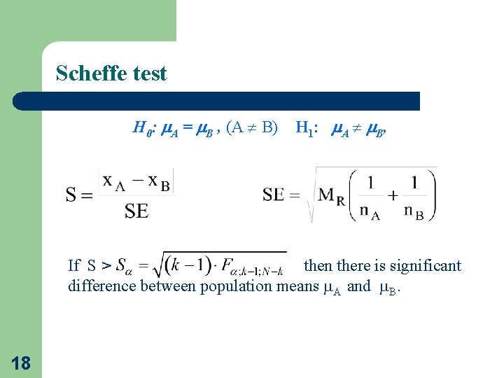
Scheffe test H 0: A = B , (A B) H 1: A B , If S > then there is significant difference between population means A and B. 18

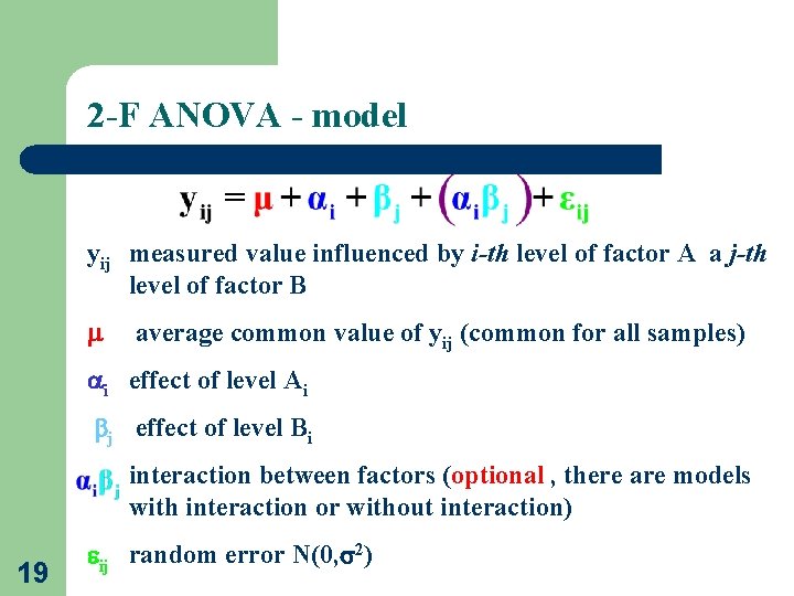
2 -F ANOVA - model yij measured value influenced by i-th level of factor A a j-th level of factor B average common value of yij (common for all samples) i effect of level Ai j effect of level Bi interaction between factors (optional , there are models with interaction or without interaction) 19 ij random error N(0, 2)

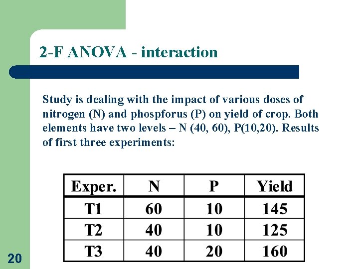
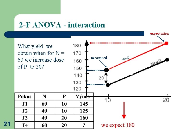
2 -F ANOVA - interaction Study is dealing with the impact of various doses of nitrogen (N) and phospforus (P) on yield of crop. Both elements have two levels – N (40, 60), P(10, 20). Results of first three experiments: 20

2 -F ANOVA - interaction expectation What yield we obtain when for N = 60 we increase dose of P to 20? 21 measured 60 N= we expect 180

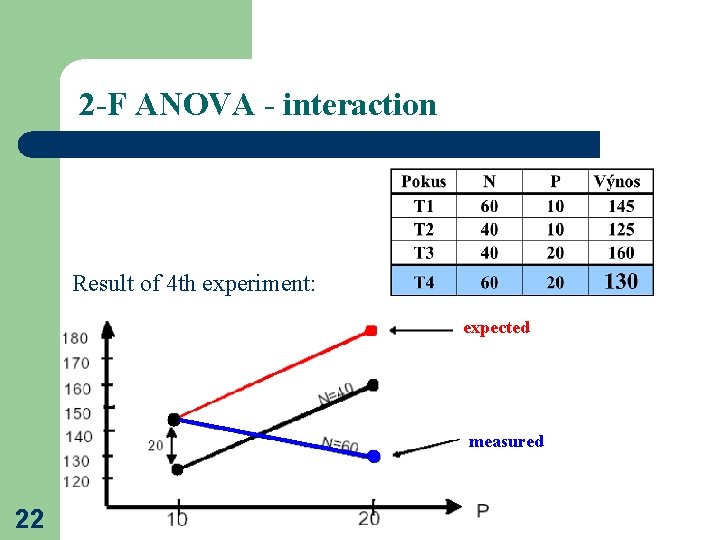
2 -F ANOVA - interaction Result of 4 th experiment: expected skutečnost measured 22

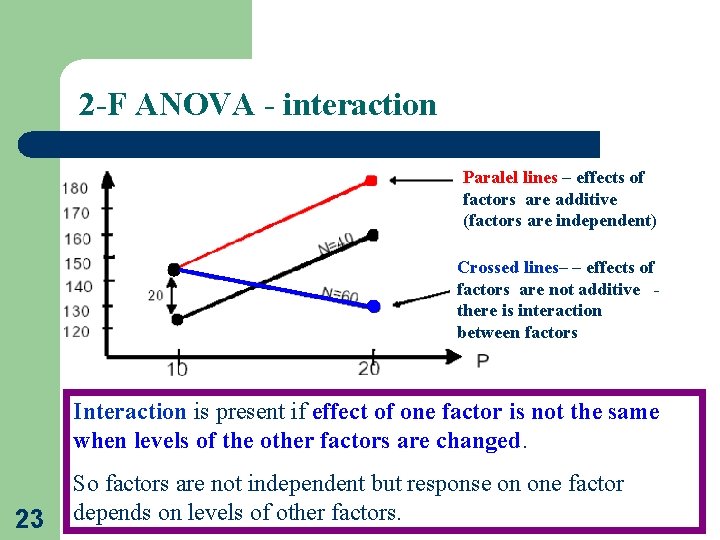
2 -F ANOVA - interaction Paralel lines – effects of factors are additive (factors are independent) Crossed lines– – effects of factors are not additive there is interaction between factors Interaction is present if effect of one factor is not the same when levels of the other factors are changed. 23 So factors are not independent but response on one factor depends on levels of other factors.

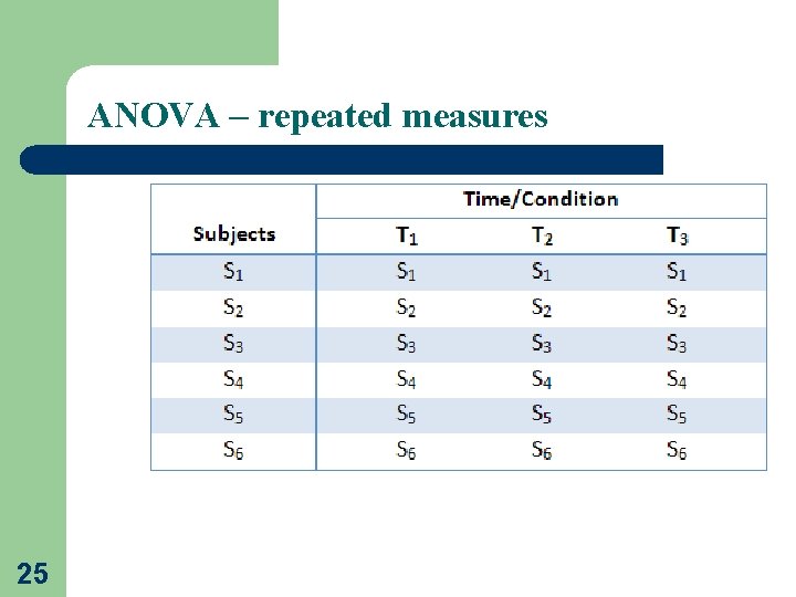
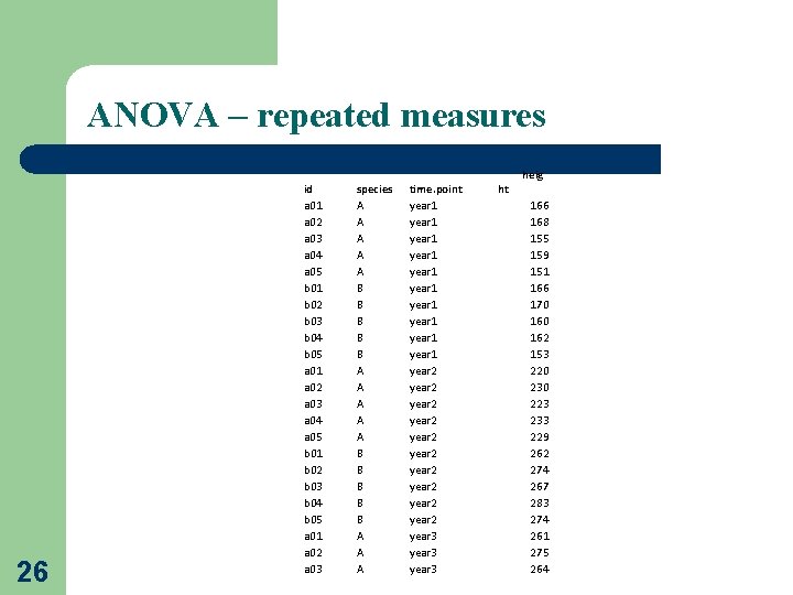
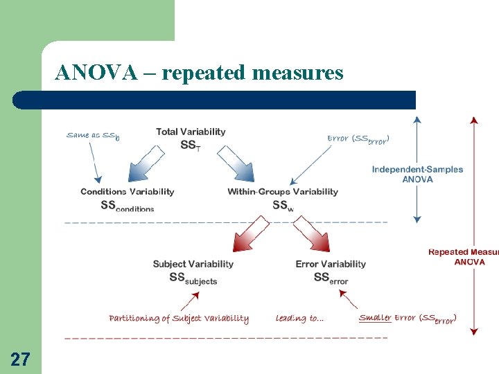
ANOVA – repeated measures A key assumption when performing fully factorial ANOVAs is that the measurements are independent. When we have repeated measures this assumption is violated, so we have to use repeated measures ANOVA 24

ANOVA – repeated measures 25

ANOVA – repeated measures 26 id a 01 a 02 a 03 a 04 a 05 b 01 b 02 b 03 b 04 b 05 a 01 a 02 a 03 species A A A A A B B B B B A A A time. point year 1 year 1 year 1 year 2 year 2 year 2 year 3 ht heig 166 168 155 159 151 166 170 162 153 220 230 223 233 229 262 274 267 283 274 261 275 264

ANOVA – repeated measures 27

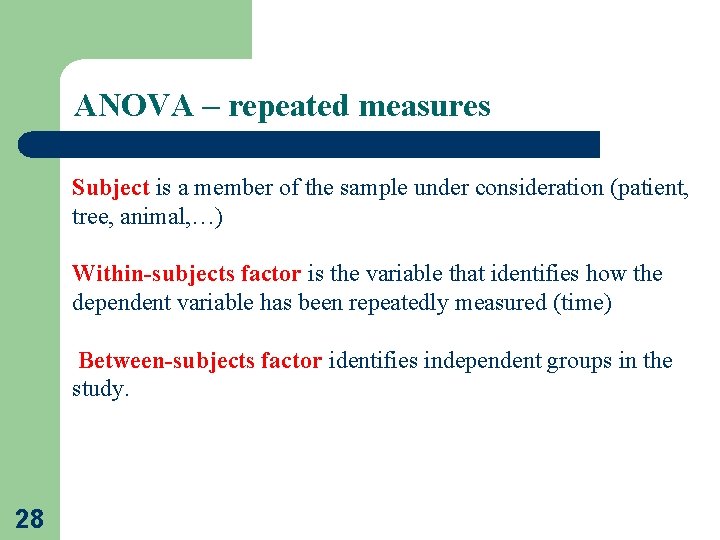
ANOVA – repeated measures Subject is a member of the sample under consideration (patient, tree, animal, …) Within-subjects factor is the variable that identifies how the dependent variable has been repeatedly measured (time) Between-subjects factor identifies independent groups in the study. 28

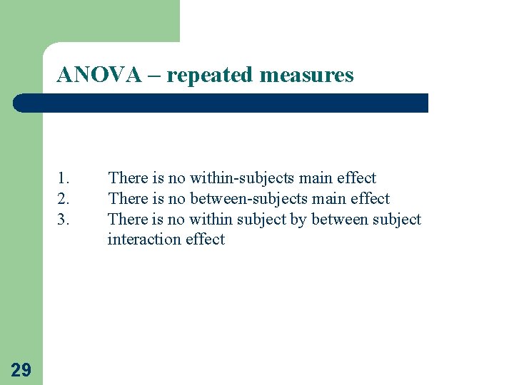
ANOVA – repeated measures 1. 2. 3. 29 There is no within-subjects main effect There is no between-subjects main effect There is no within subject by between subject interaction effect

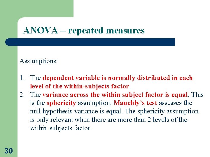
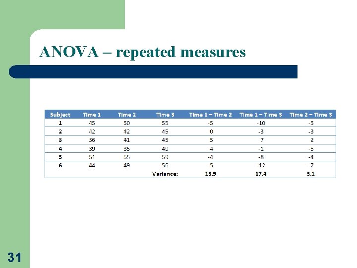
ANOVA – repeated measures Assumptions: 1. The dependent variable is normally distributed in each level of the within-subjects factor. 2. The variance across the within subject factor is equal. This is the sphericity assumption. Mauchly’s test assesses the null hypothesis variance is equal. The sphericity assumption is only relevant when there are more than 2 levels of the within subjects factor. 30

ANOVA – repeated measures 31

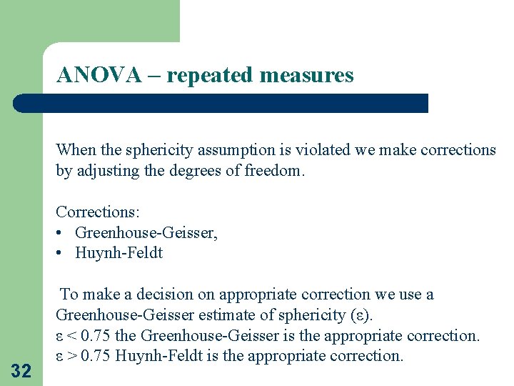
ANOVA – repeated measures When the sphericity assumption is violated we make corrections by adjusting the degrees of freedom. Corrections: • Greenhouse-Geisser, • Huynh-Feldt 32 To make a decision on appropriate correction we use a Greenhouse-Geisser estimate of sphericity (ε). ε < 0. 75 the Greenhouse-Geisser is the appropriate correction. ε > 0. 75 Huynh-Feldt is the appropriate correction.

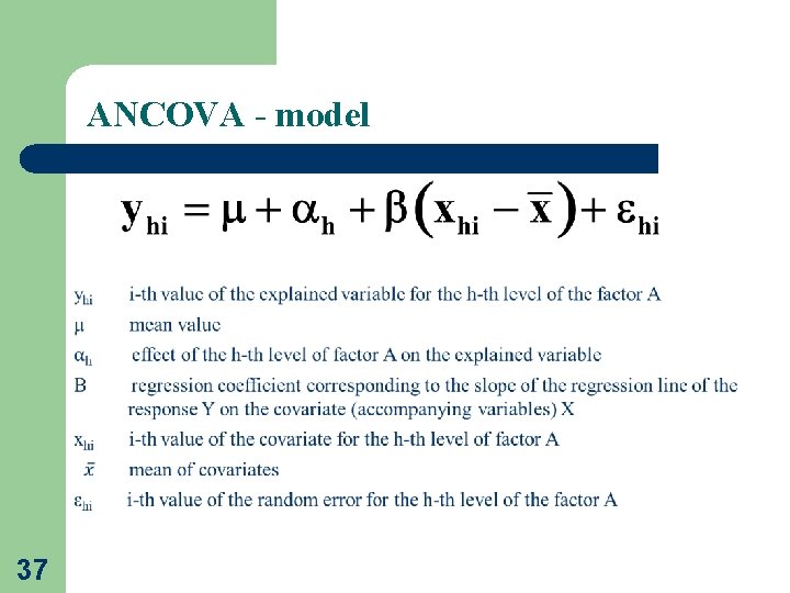
Analysis of Covariance (ANCOVA) The Analysis of Covariance (ANCOVA) is used to compare means of an outcome variable between two or more groups taking into account (or to correct for) variability of other variables, called covariates. ANCOVA allows to compare the adjusted means of two or more independent groups 33

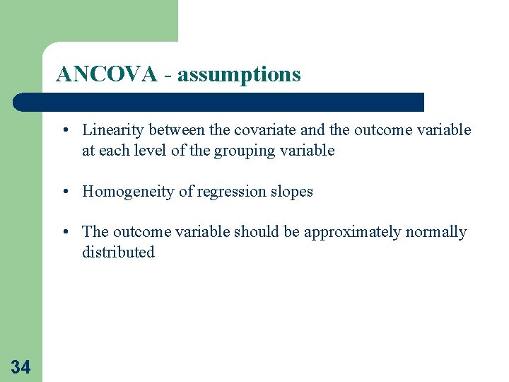
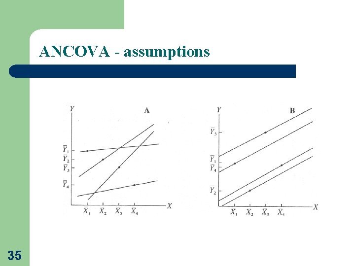
ANCOVA - assumptions • Linearity between the covariate and the outcome variable at each level of the grouping variable • Homogeneity of regression slopes • The outcome variable should be approximately normally distributed 34

ANCOVA - assumptions 35

ANCOVA - assumptions 36

ANCOVA - model 37

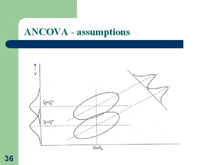
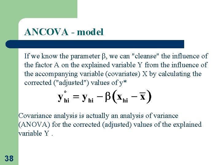
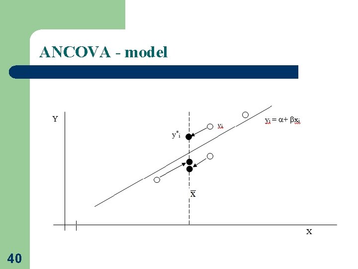
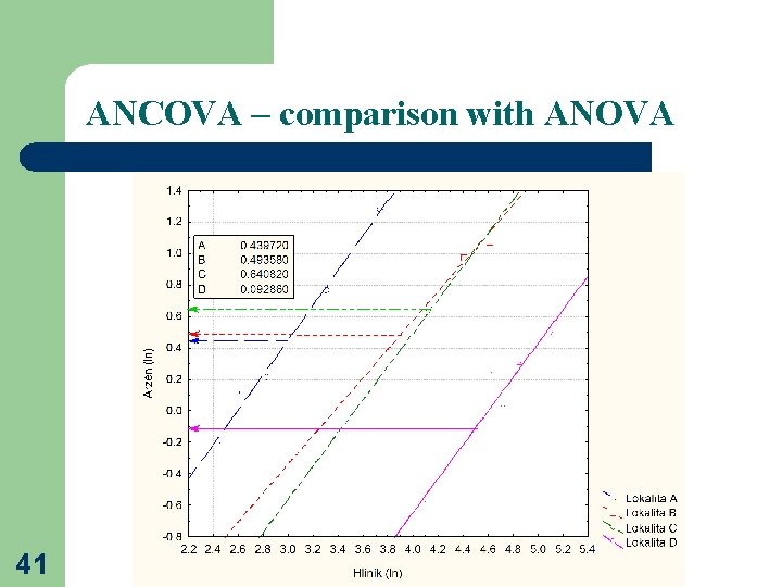
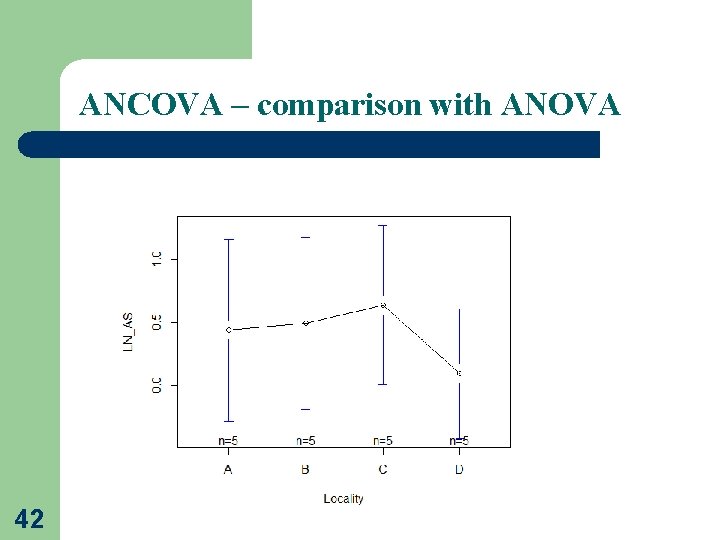
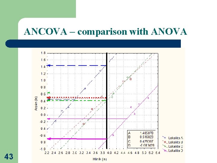
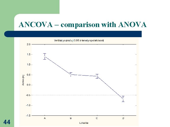
ANCOVA - model If we know the parameter β, we can "cleanse" the influence of the factor A on the explained variable Y from the influence of the accompanying variable (covariates) X by calculating the corrected ("adjusted") values of y* Covariance analysis is actually an analysis of variance (ANOVA) for the corrected (adjusted) values of the explained variable Y. 38

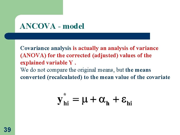
ANCOVA - model Covariance analysis is actually an analysis of variance (ANOVA) for the corrected (adjusted) values of the explained variable Y. We do not compare the original means, but the means converted (recalculated) to the mean value of the covariate 39

ANCOVA - model 40

ANCOVA – comparison with ANOVA 41

ANCOVA – comparison with ANOVA 42

ANCOVA – comparison with ANOVA 43

ANCOVA – comparison with ANOVA 44