Analysis of twoway tables Data analysis for twoway

Objectives (IPS chapter 9. 1) Data analysis for two-way tables p Two-way tables p Marginal distributions p Relationships between categorical variables p Conditional distributions p Simpson’s paradox

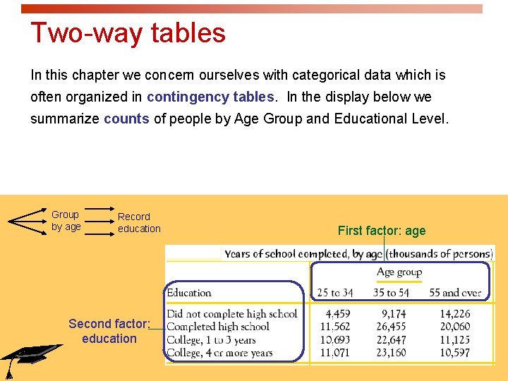
Two-way tables In this chapter we concern ourselves with categorical data which is often organized in contingency tables. In the display below we summarize counts of people by Age Group and Educational Level. Group by age Record education Second factor: education First factor: age

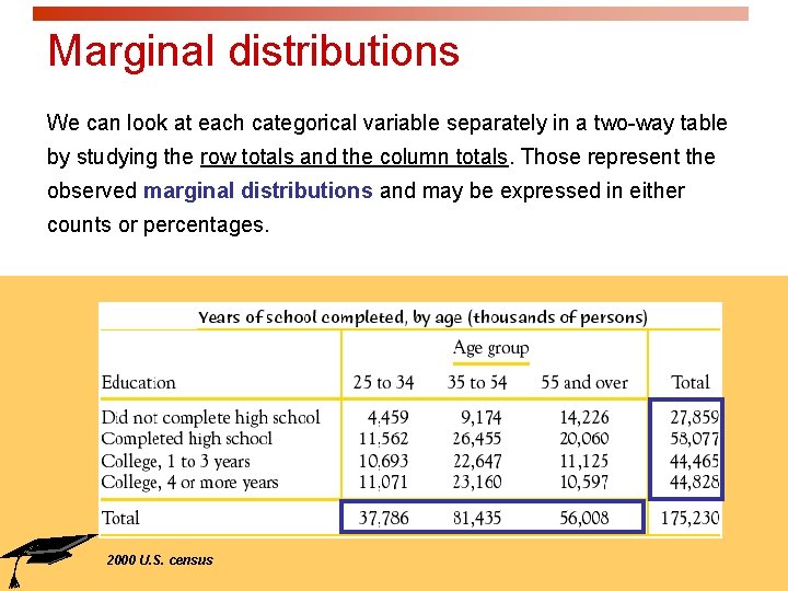
Marginal distributions We can look at each categorical variable separately in a two-way table by studying the row totals and the column totals. Those represent the observed marginal distributions and may be expressed in either counts or percentages. 2000 U. S. census

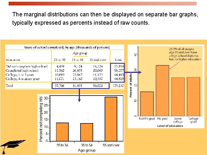
The marginal distributions can then be displayed on separate bar graphs, typically expressed as percents instead of raw counts.

Relationships between categorical variables The marginal distributions summarize each categorical variable independently. But, the two-way table describes the relationship between both categorical variables. The cells of a two-way table represent the intersection, or joint occurrence of each level of a categorical factor with each level of the other categorical factor. Because counts can be confusing (for instance, one level of one factor might be much less represented than the other levels), we might prefer to display proportions for the corresponding cells and margins.

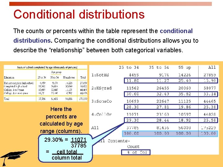
Conditional distributions The counts or percents within the table represent the conditional distributions. Comparing the conditional distributions allows you to describe the “relationship” between both categorical variables. Here the percents are calculated by age range (columns). 29. 30% = 11071 37785 = cell total. column total

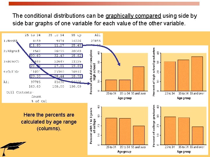
The conditional distributions can be graphically compared using side by side bar graphs of one variable for each value of the other variable. Here the percents are calculated by age range (columns).

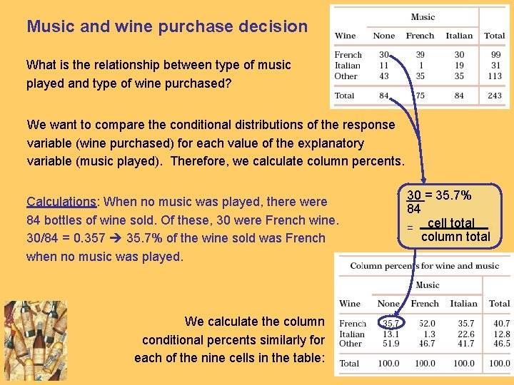
Music and wine purchase decision What is the relationship between type of music played and type of wine purchased? We want to compare the conditional distributions of the response variable (wine purchased) for each value of the explanatory variable (music played). Therefore, we calculate column percents. Calculations: When no music was played, there were 84 bottles of wine sold. Of these, 30 were French wine. 30/84 = 0. 357 35. 7% of the wine sold was French when no music was played. We calculate the column conditional percents similarly for each of the nine cells in the table: 30 = 35. 7% 84 = cell total. column total

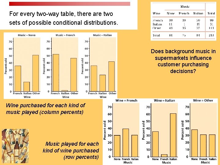
For every two-way table, there are two sets of possible conditional distributions. Does background music in supermarkets influence customer purchasing decisions? Wine purchased for each kind of music played (column percents) Music played for each kind of wine purchased (row percents)

Simpson’s paradox An association or comparison that holds for all of several groups can reverse direction when the data are combined (aggregated) to form a single group. This reversal is called Simpson’s paradox. On the surface, Hospital B would seem to have a better record. Example: Hospital death rates But once patient condition is taken into account, we see that hospital A has in fact a better record for both patient conditions (good and poor). Here patient condition was the lurking variable.