Analysis of TABASSUM KHAN UNIVERSITY OF SCIENCE AND

Analysis of TABASSUM KHAN UNIVERSITY OF SCIENCE AND TECHNOLOGY, CHINA
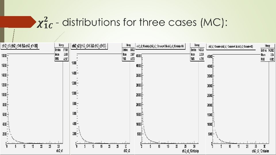
 <2. 4")
MOTIVATION: Final state (4. 5± 1. 5) <2. 4

Boss version and Datasets: Boss 6. 6. 4 p 03 (2009 DATA with run no. for mc {-8093, 0, -9025}) 106 M Ψ′ experimental data 106 M Ψ′ inclusive MC sample (2012 DATA with run no. for mc {-25338, 0, -27090}) 340 M Ψ′ experimental data 400 M Ψ′ inclusive MC sample

Selection criteria:
: 2009 DATA 2012 DATA Cut")
Comparison of cut-efficiency for 2009 and 2012 MC(ihep cluster): 2009 DATA 2012 DATA Cut efficiency for 2009 MC Cut efficiency for 2012 MC Total number 402000 n. Good>=4 287539 266548 71. 52% 66. 30% Pass Pid 255172 233784 88. 74% 87. 70% Ks selection 233153 213172 91. 37% 91. 18% Pass 1 C 227525 207752 97. 58% 97. 45%
; Quality check of data:")
Float_t rightmaxdata 09 = mks 0_histre 09 ->Get. Maximum(); Quality check of data: Float_t rightmaxmc 09 = mks 0_histmc 09 ->Get. Maximum(); Float_t rightmaxdata 12 = mks 0_histre 12 ->Get. Maximum(); Float_t rightmaxmc 12 = mks 0_histmc 12 ->Get. Maximum(); mks 0_histre 09 ->Scale(rightmaxmc 09/rightmaxdata 09); mks 0_histre 12 ->Scale(rightmaxmc 12/rightmaxdata 12);

A comparison of truth information of total momentum of proton for 2009 and 2012 MC:

Comparison of efficiency curve:

A comparison of Mdc. Kal. Trk information for total momentum of proton for 2009 and 2012 MC:

A comparison of efficiency curve:

Comparison of total momentum for proton for MC and Real data for 2009 and 2012:
*1. 0/hpproton_mc->Integral());")
hpproton_mc->Scale(hpproton_real->Integral()*1. 0/hpproton_mc->Integral());
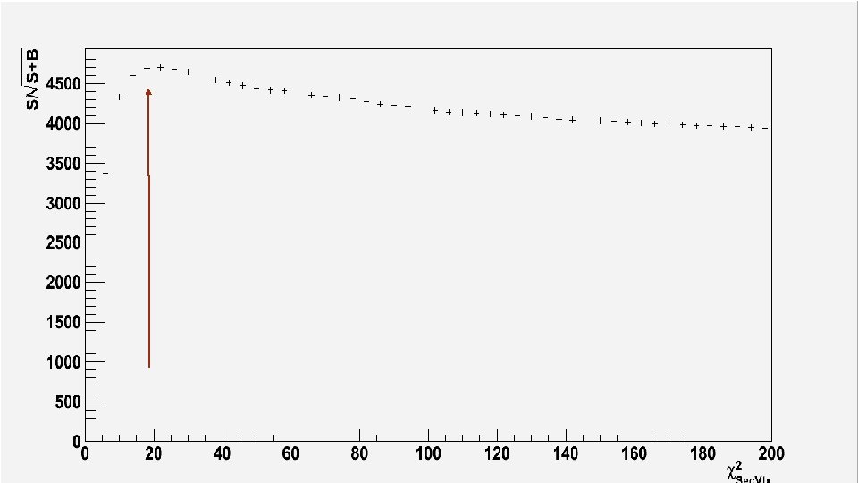
<20: Scaling: chisq_histmc->Scale(rightmaxdata/rightmaxmc); chisq_histincl>Scale(rightmaxdata/rightmaxincl);")
χ2(Second. Vertex. Fit)<20: Scaling: chisq_histmc->Scale(rightmaxdata/rightmaxmc); chisq_histincl>Scale(rightmaxdata/rightmaxincl);
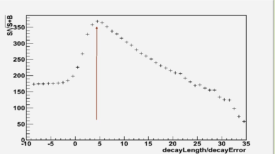
/double(decay_histmc->Get. Entries())); decay_histincl->Scale(rightmaxdata/rightmaxincl);")
decay. Length/decaylength. Error: Scaling: decay_histmc->Scale(decay_histre->Get. Entries()/double(decay_histmc->Get. Entries())); decay_histincl->Scale(rightmaxdata/rightmaxincl);
<20 L/ϬL>2 m_mks 0 - 0. 49767 <")
Cuts applied: Φ-mass<1. 10 χ2(Second. Vertex. Fit)<20 L/ϬL>2 m_mks 0 - 0. 49767 < 0. 007 Scaling: chisq 1 Cfit_histmc->Scale(rightmaxdata/rightmaxmc); chisq 1 Cfit_histincl->Scale(rightmaxdata/rightmaxincl);

Maximum value get after optimization is 4
 – 0. 49767|<7 Me. V/c 2 Scaling: mks 0_histmc-> Scale(mks 0_histre->Get. Maximum()/mks 0_histmc->Get.")
|M(π+π-) – 0. 49767|<7 Me. V/c 2 Scaling: mks 0_histmc-> Scale(mks 0_histre->Get. Maximum()/mks 0_histmc->Get. Maximum()); mks 0_histincl -> Scale(mks 0_histre->Get. Maximum()/mks 0_histincl->Get. Maximum());

Maximum value get after optimization is 0. 004
: Scaling: chisq 1 Cfit_histmc->Scale(rightmaxdata/rightmaxmc); chisq 1 Cfit_histincl->Scale(rightmaxdata/rightmaxincl);")
ϕ- Mass distribution plot (with general cuts): Scaling: chisq 1 Cfit_histmc->Scale(rightmaxdata/rightmaxmc); chisq 1 Cfit_histincl->Scale(rightmaxdata/rightmaxincl);
: Scaling: chisq 1 Cfit_histmc->Scale(rightmaxdata/rightmaxmc); chisq 1 Cfit_histincl->Scale(rightmaxdata/rightmaxincl);")
ϕ- Mass distribution plot (with optimized cuts): Scaling: chisq 1 Cfit_histmc->Scale(rightmaxdata/rightmaxmc); chisq 1 Cfit_histincl->Scale(rightmaxdata/rightmaxincl);

Doing comparison of L/ϬL>2 and L/ϬL>4 : Cut efficiency for L/ϬL>2 is 84. 65% Cut efficiency for L/ϬL>4 is 74. 66%
 – 0. 49767|<7 Me. V/c 2 L/ϬL>4 L/ϬL>2 Scaling: mks 0_histmc-> Scale(mks 0_histre->Get.")
|M(π+π-) – 0. 49767|<7 Me. V/c 2 L/ϬL>4 L/ϬL>2 Scaling: mks 0_histmc-> Scale(mks 0_histre->Get. Maximum()/mks 0_histmc->Get. Maximum()); mks 0_histincl -> Scale(mks 0_histre->Get. Maximum()/mks 0_histincl->Get. Maximum());

Topology analysis:
:")
Background study(with general cuts):
:")
Background study(with optimized cuts):

Background study: Cut efficiency = 69. 73% Cut efficiency = 84. 50% Not significant

ϕ Final fitting results of - signal
: Argus= Cuts Applied: phimass <1. 10 m_chi")
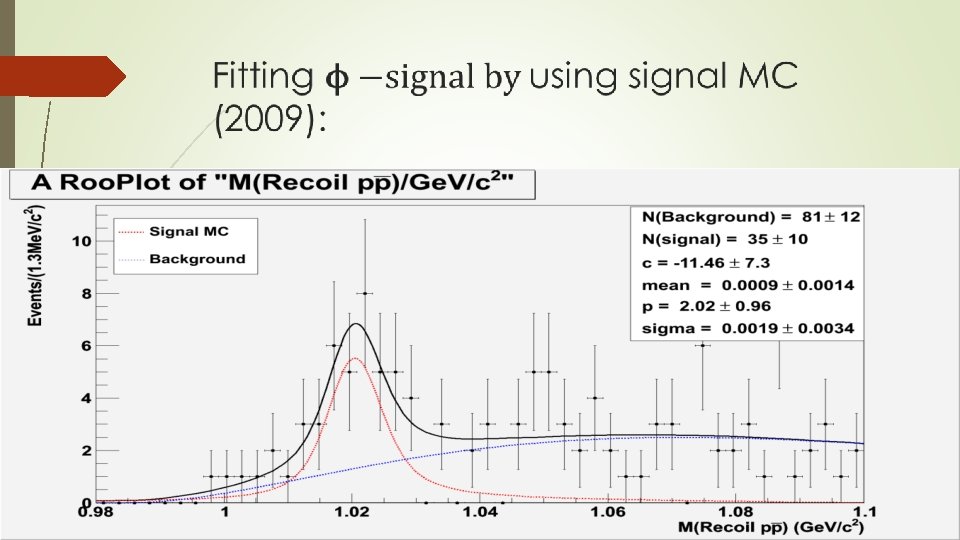
Important parameters for fitting ϕ-signal (Unbinned method): Argus= Cuts Applied: phimass <1. 10 m_chi 2 < 4 decayle > 2 m_chisqvtxnd<20 |m_mks 0 - 0. 49767| < 0. 005

ϕ Fitting of -signal for 2009 data

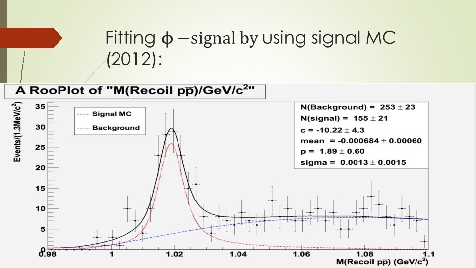
ϕ Fitting of -signal for 2012 data

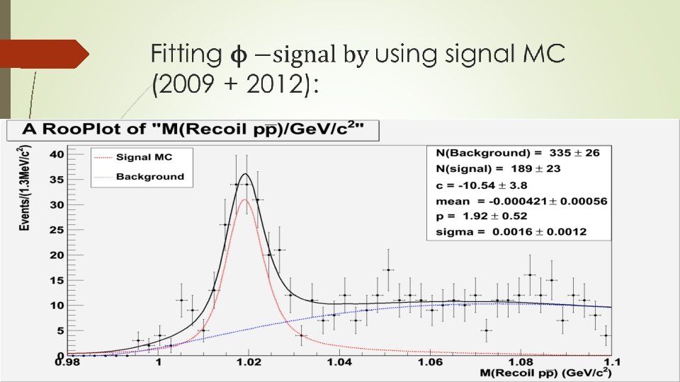
ϕ Fitting of -signal for 2009+2012 data
: Argus= Cuts Applied: phimass <1.")
Important parameters for fitting of ϕ- signal (binned method): Argus= Cuts Applied: phimass <1. 10 m_chi 2 < 4 decayle > 2 m_chisqvtxnd<20 |m_mks 0 - 0. 49767| < 0. 005
: 2009 MC Cut")
Cut flow of MC (total number of MC generated = 402000): 2009 MC Cut flow for 2009 MC 2012 MC 227525 207752 435277 226982 207194 434176 160062 136898 144009 304071 122208 259106 126160 112015 238175 Total Number of events (after PID) (mks 00. 49767)<0. 005 116520 28. 98% 103001 Cut flow for 2012 MC 25. 62% Combined data(2009+2012) 219521 Cut flow for 2009+2012 27. 30%

Branching fraction calculation

For 2009 data:

-mass distribution plots
 - mass distribution for 2009 data")
Comparison between 2009 and 2012 data(using general cuts) - mass distribution for 2009 data - mass distribution for 2012 data

- mass distribution plot for combined data of 2009 and 2012 (using general cuts):
 - mass distribution for 2009 data")
Comparison between 2009 and 2012 data(using optimized cuts) - mass distribution for 2009 data - mass distribution for 2012 data

- mass distribution plot for combined data of 2009 and 2012 (using optimized cuts):

Background Estimation: The previous plots also show the background estimation, there is no signal for inclusive MC. Looking at the shape of blue line, it represents the estimated background, that there is no peak along the phi-mass region. So there is no peaking background. .
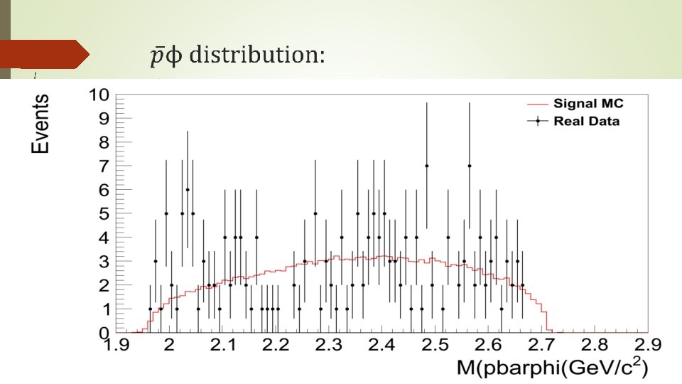
 * 1. 0 / pphi_hist->Integral());")
pϕ distribution: pphi_hist->Scale(pphi_histre->Integral() * 1. 0 / pphi_hist->Integral());

pϕ distribution in side-band region: N 1=48. 963 , N 2= 64. 271 ; pphi_histre_sd->Scale(N 1/N 2);

Analysis of TABASSUM KHAN UNIVERSITY OF SCIENCE AND TECHNOLOGY, CHINA

Selection criteria:
: 2012 DATA")
Cut-efficiency for 2012 MC for 1000 no. of events (ihep cluster): 2012 DATA Cut efficiency for 2012 MC Total number 1000 n. Good>=3 824 82. 4% Pass Pid 686 83. 25% Pass 1 C__case 1 683 99. 56% Pass 1 C_case 2 680 99. 56% Pass 4 C_case 3 658 96. 76% Cut efficiency for 2012 MC Total number 1000 n. Good>=3 824 82. 4% Pass Pid 686 83. 25% Pass 1 C__case 1 683 99. 56% Pass 1 C_case 2 680 99. 56% Pass 1 C_case 3 677 99. 56% Using 1 C-kinematic fit has improved the efficiency.
: 2012 DATA")
Cut-efficiency for 2012 MC for 402000 no. of events (ihep cluster): 2012 DATA Cut efficiency for 2012 MC Total number 402000 n. Good>=3 325919 81. 07% Pass Pid 265672 81. 51% Pass 1 C__case 1 264942 99. 72% Pass 1 C_case 2 264330 99. 76% Pass 1 C_case 3 262425 99. 27%

Phi-mass distribution plot:

Next work: Run Real data Compare mc and real data Optimization Background study

- Slides: 59