Analysis of Quantitative data Students ttest Anne SegondsPichon

Analysis of Quantitative data Student’s t-test Anne Segonds-Pichon v 2020 -12

Comparison between 2 groups

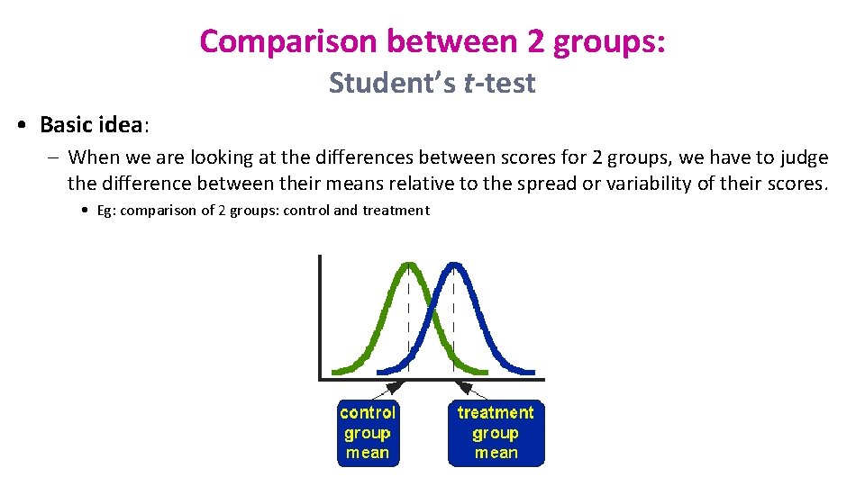
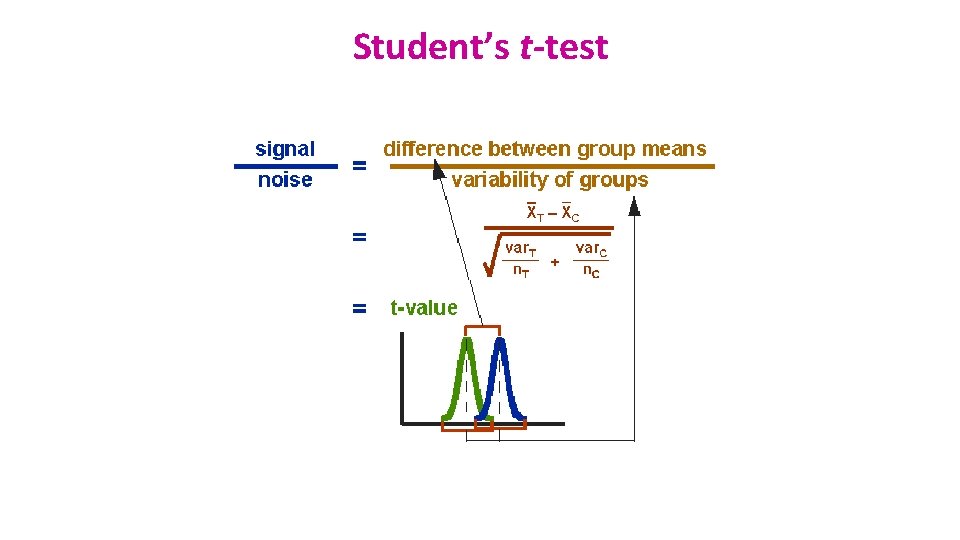
Comparison between 2 groups: Student’s t-test • Basic idea: – When we are looking at the differences between scores for 2 groups, we have to judge the difference between their means relative to the spread or variability of their scores. • Eg: comparison of 2 groups: control and treatment

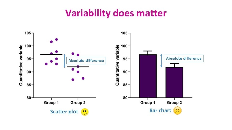
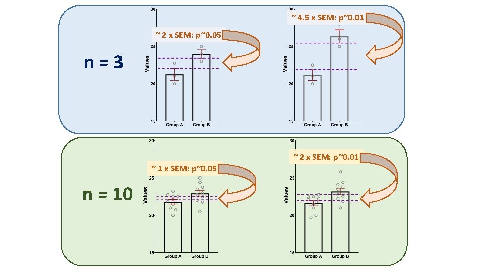
Variability does matter Absolute difference Scatter plot Absolute difference Bar chart

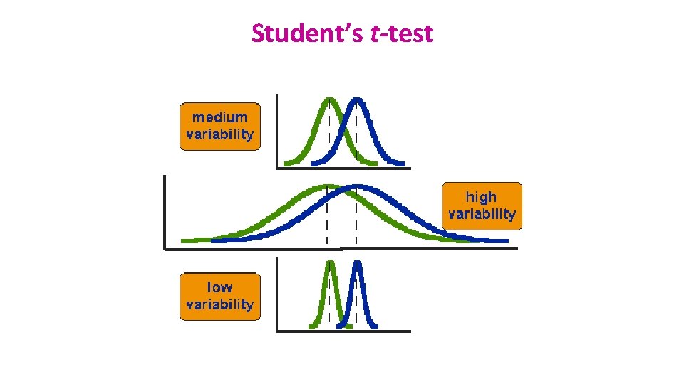
Student’s t-test

Student’s t-test

~ 4. 5 x SEM: p~0. 01 ~ 2 x SEM: p~0. 05 n=3 ~ 2 x SEM: p~0. 01 ~ 1 x SEM: p~0. 05 n = 10

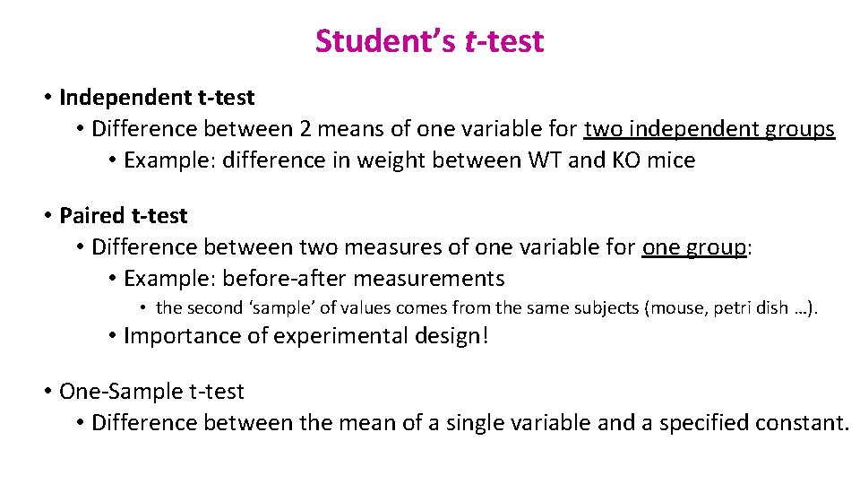
Student’s t-test • Independent t-test • Difference between 2 means of one variable for two independent groups • Example: difference in weight between WT and KO mice • Paired t-test • Difference between two measures of one variable for one group: • Example: before-after measurements • the second ‘sample’ of values comes from the same subjects (mouse, petri dish …). • Importance of experimental design! • One-Sample t-test • Difference between the mean of a single variable and a specified constant.

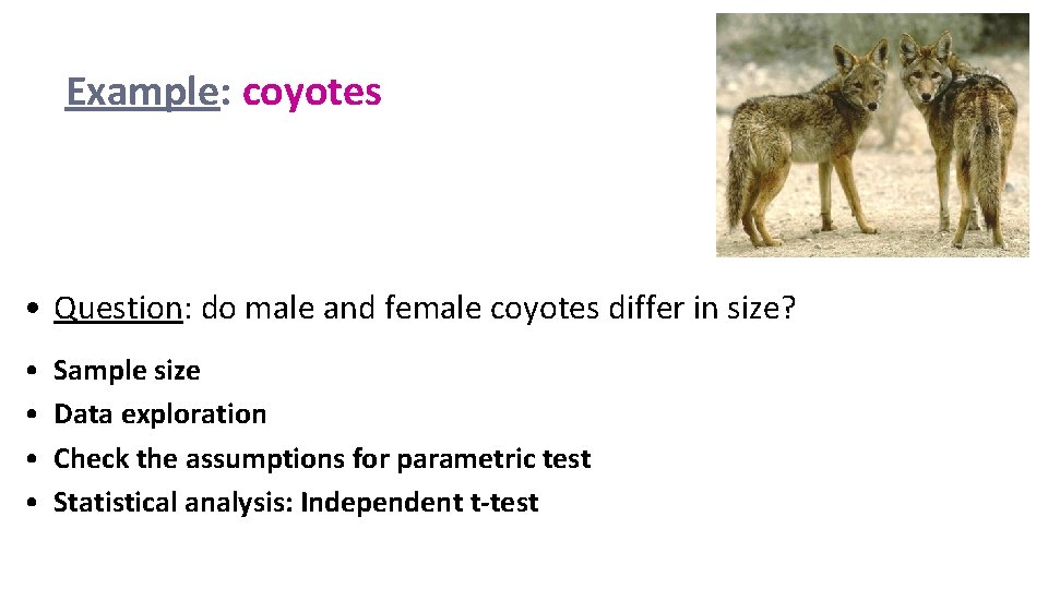
Example: coyotes • Question: do male and female coyotes differ in size? • • Sample size Data exploration Check the assumptions for parametric test Statistical analysis: Independent t-test

Exercise 3: Power analysis • Example case: No data from a pilot study but we have found some information in the literature. In a study run in similar conditions as in the one we intend to run, male coyotes were found to measure: 92 cm +/- 7 cm (SD). We expect a 5% difference between genders. • smallest biologically meaningful difference power. t. test(n = NULL, delta = NULL, sd = 1, sig. level = NULL, power = NULL, type = c("two. sample", "one. sample", "paired"), alternative = c("two. sided", "one. sided"))

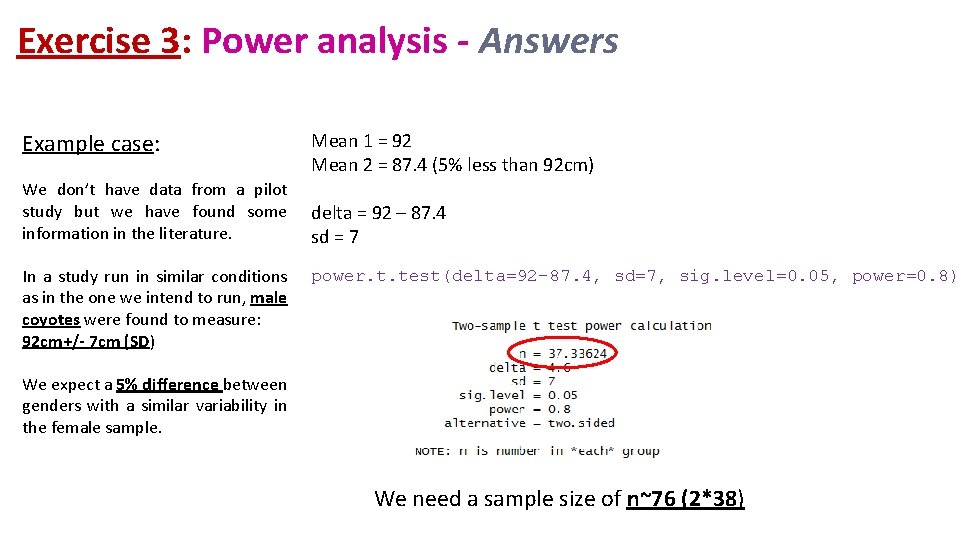
Exercise 3: Power analysis - Answers Example case: We don’t have data from a pilot study but we have found some information in the literature. In a study run in similar conditions as in the one we intend to run, male coyotes were found to measure: 92 cm+/- 7 cm (SD) Mean 1 = 92 Mean 2 = 87. 4 (5% less than 92 cm) delta = 92 – 87. 4 sd = 7 power. t. test(delta=92 -87. 4, sd=7, sig. level=0. 05, power=0. 8) We expect a 5% difference between genders with a similar variability in the female sample. We need a sample size of n~76 (2*38)

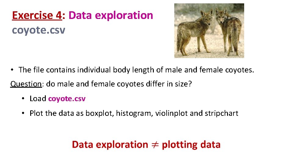
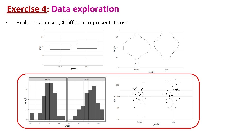
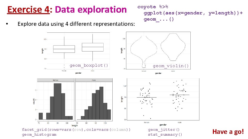
Exercise 4: Data exploration coyote. csv • The file contains individual body length of male and female coyotes. Question: do male and female coyotes differ in size? • Load coyote. csv • Plot the data as boxplot, histogram, violinplot and stripchart

Exercise 4: Data exploration • Explore data using 4 different representations:

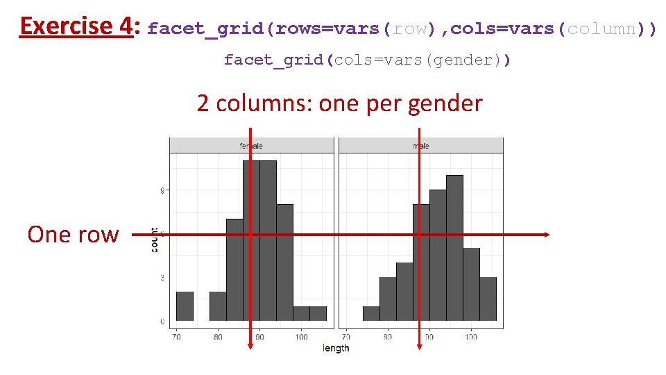
Exercise 4: facet_grid(rows=vars(row), cols=vars(column)) facet_grid(cols=vars(gender)) 2 columns: one per gender One row

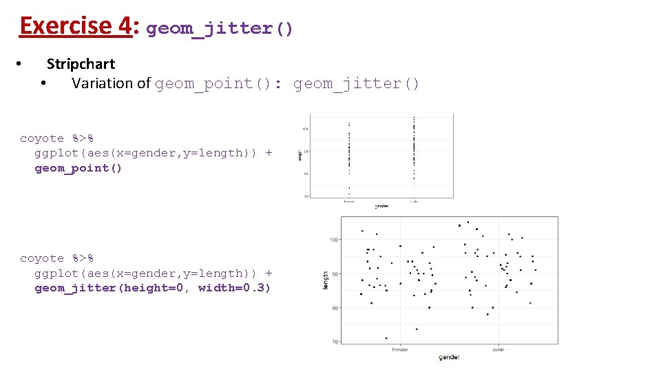
Exercise 4: geom_jitter() • Stripchart • Variation of geom_point(): geom_jitter() coyote %>% ggplot(aes(x=gender, y=length)) + geom_point() coyote %>% ggplot(aes(x=gender, y=length)) + geom_jitter(height=0, width=0. 3)

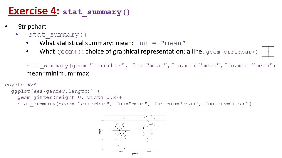
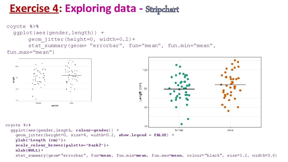
Exercise 4: stat_summary() • Stripchart • stat_summary() • What statistical summary: mean: fun = "mean" • What geom(): choice of graphical representation: a line: geom_errorbar() stat_summary(geom="errorbar", fun="mean", fun. min="mean", fun. max="mean") mean=minimum=max coyote %>% ggplot(aes(gender, length)) + geom_jitter(height=0, width=0. 2)+ stat_summary(geom= "errorbar", fun="mean", fun. min="mean", fun. max="mean")

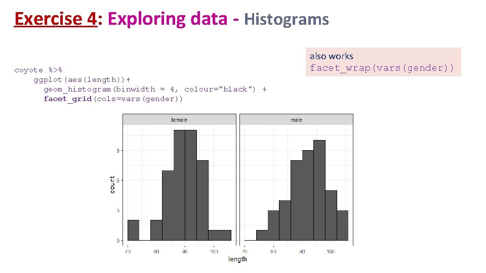
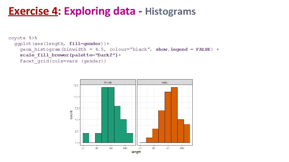
Exercise 4: Data exploration • Explore data using 4 different representations: geom_boxplot() facet_grid(rows=vars(row), cols=vars(column)) geom_histogram coyote %>% ggplot(aes(x=gender, y=length))+ geom_. . . () geom_violin() geom_jitter() stat_summary() Have a go!

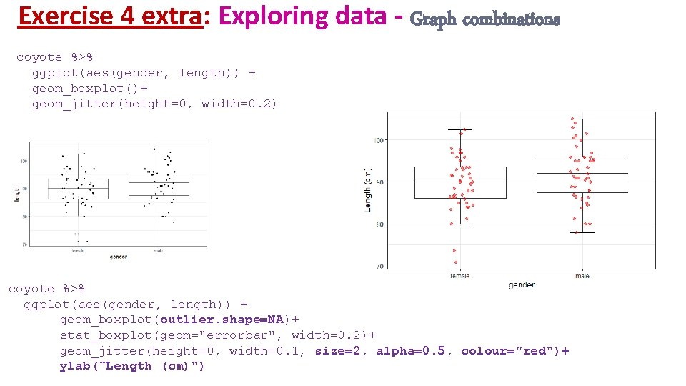
Exercise 4: Exploring data - Stripchart coyote %>% ggplot(aes(gender, length)) + geom_jitter(height=0, width=0. 2)+ stat_summary(geom= "errorbar", fun="mean", fun. min="mean", fun. max="mean") coyote %>% ggplot(aes(gender, length, colour=gender)) + geom_jitter(height=0, size=4, width=0. 2, show. legend = FALSE) + ylab("Length (cm)")+ scale_colour_brewer(palette="Dark 2")+ xlab(NULL)+ stat_summary(geom="errorbar", fun=mean, fun. min=mean, fun. max=mean, colour="black", size=1. 2, width=0. 6)

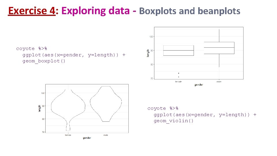
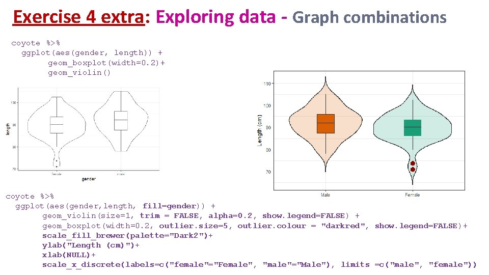
Exercise 4: Exploring data - Boxplots and beanplots coyote %>% ggplot(aes(x=gender, y=length)) + geom_boxplot() coyote %>% ggplot(aes(x=gender, y=length)) + geom_violin()

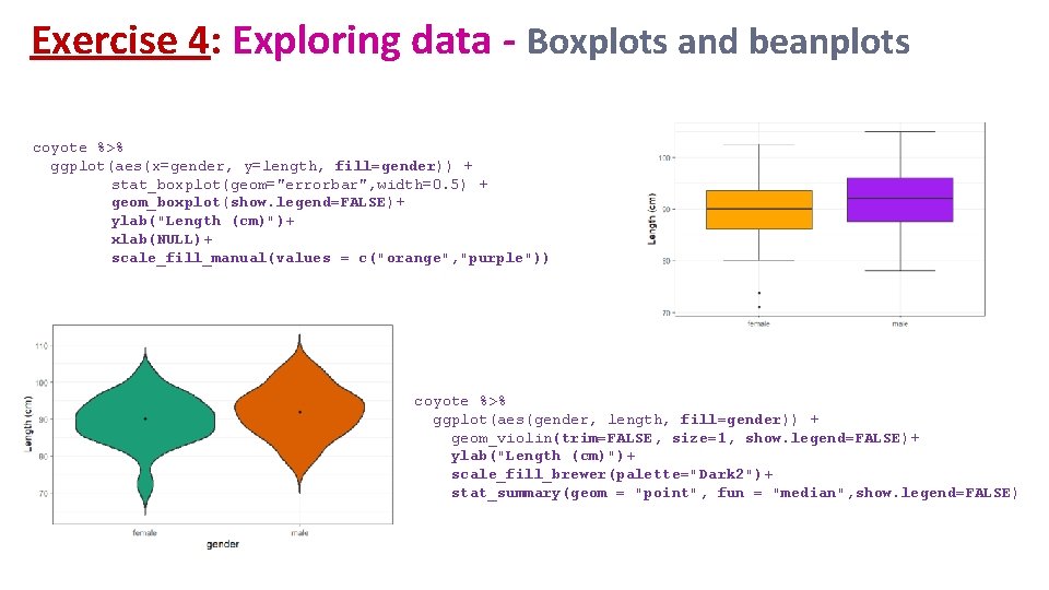
Exercise 4: Exploring data - Boxplots and beanplots coyote %>% ggplot(aes(x=gender, y=length, fill=gender)) + stat_boxplot(geom="errorbar", width=0. 5) + geom_boxplot(show. legend=FALSE)+ ylab("Length (cm)")+ xlab(NULL)+ scale_fill_manual(values = c("orange", "purple")) coyote %>% ggplot(aes(gender, length, fill=gender)) + geom_violin(trim=FALSE, size=1, show. legend=FALSE)+ ylab("Length (cm)")+ scale_fill_brewer(palette="Dark 2")+ stat_summary(geom = "point", fun = "median", show. legend=FALSE)

Exercise 4: Exploring data - Histograms coyote %>% ggplot(aes(length))+ geom_histogram(binwidth = 4, colour="black") + facet_grid(cols=vars(gender)) also works facet_wrap(vars(gender))

Exercise 4: Exploring data - Histograms coyote %>% ggplot(aes(length, fill=gender))+ geom_histogram(binwidth = 4. 5, colour="black", show. legend = FALSE) + scale_fill_brewer(palette="Dark 2")+ facet_grid(cols=vars (gender))

Exercise 4 extra: Exploring data - Graph combinations coyote %>% ggplot(aes(gender, length)) + geom_boxplot(width=0. 2)+ geom_violin() coyote %>% ggplot(aes(gender, length, fill=gender)) + geom_violin(size=1, trim = FALSE, alpha=0. 2, show. legend=FALSE) + geom_boxplot(width=0. 2, outlier. size=5, outlier. colour = "darkred", show. legend=FALSE)+ scale_fill_brewer(palette="Dark 2")+ ylab("Length (cm)")+ xlab(NULL)+ scale_x_discrete(labels=c("female"="Female", "male"="Male"), limits =c("male", "female"))

Exercise 4 extra: Exploring data - Graph combinations coyote %>% ggplot(aes(gender, length)) + geom_boxplot()+ geom_jitter(height=0, width=0. 2) coyote %>% ggplot(aes(gender, length)) + geom_boxplot(outlier. shape=NA)+ stat_boxplot(geom="errorbar", width=0. 2)+ geom_jitter(height=0, width=0. 1, size=2, alpha=0. 5, colour="red")+ ylab("Length (cm)")

Checking the assumptions

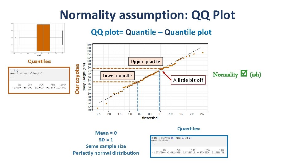
Normality assumption: QQ Plot Quantiles: Our coyotes QQ plot= Quantile – Quantile plot Upper quartile Lower quartile Mean = 0 SD = 1 Same sample size Perfectly normal distribution A little bit off Quantiles: Normality (ish)

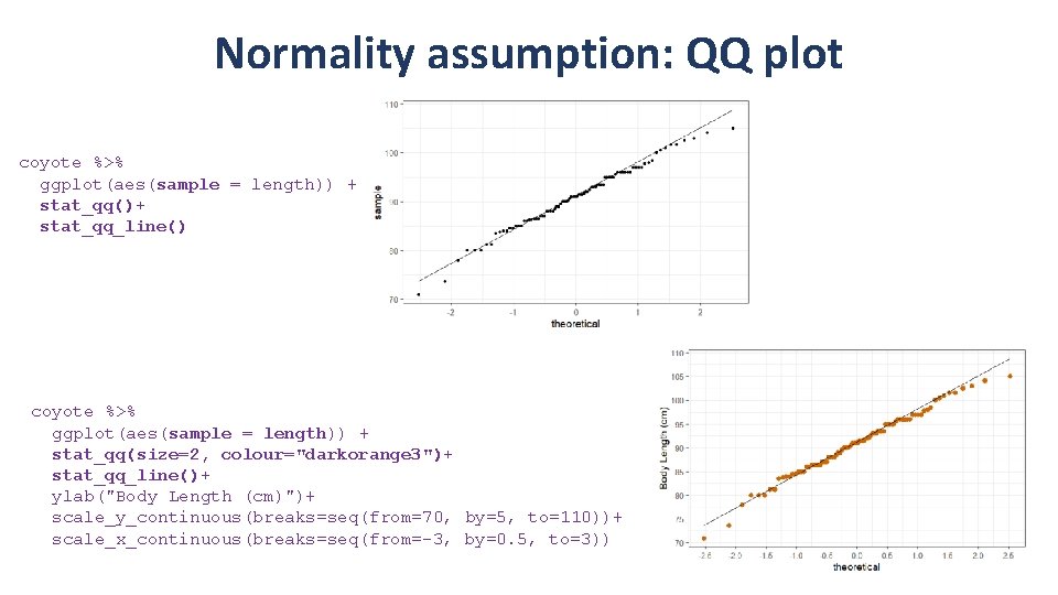
Normality assumption: QQ plot coyote %>% ggplot(aes(sample = length)) + stat_qq()+ stat_qq_line() coyote %>% ggplot(aes(sample = length)) + stat_qq(size=2, colour="darkorange 3")+ stat_qq_line()+ ylab("Body Length (cm)")+ scale_y_continuous(breaks=seq(from=70, by=5, to=110))+ scale_x_continuous(breaks=seq(from=-3, by=0. 5, to=3))

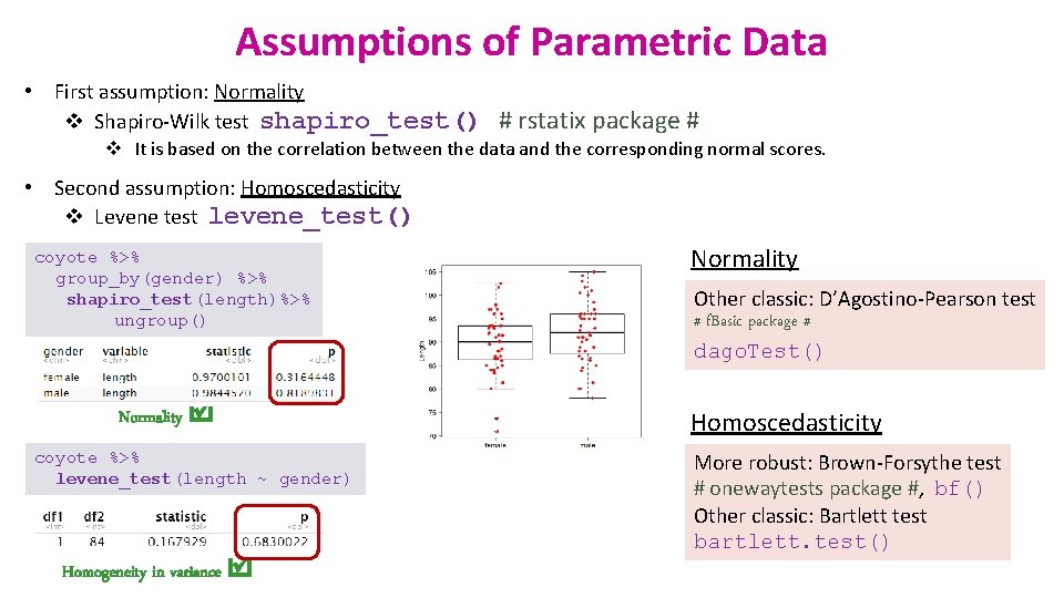
Assumptions of Parametric Data • First assumption: Normality v Shapiro-Wilk test shapiro_test() # rstatix package # v It is based on the correlation between the data and the corresponding normal scores. • Second assumption: Homoscedasticity v Levene test levene_test() coyote %>% group_by(gender) %>% shapiro_test(length)%>% ungroup() Normality coyote %>% levene_test(length ~ gender) Homogeneity in variance Normality Other classic: D’Agostino-Pearson test # f. Basic package # dago. Test() Homoscedasticity More robust: Brown-Forsythe test # onewaytests package #, bf() Other classic: Bartlett test bartlett. test()

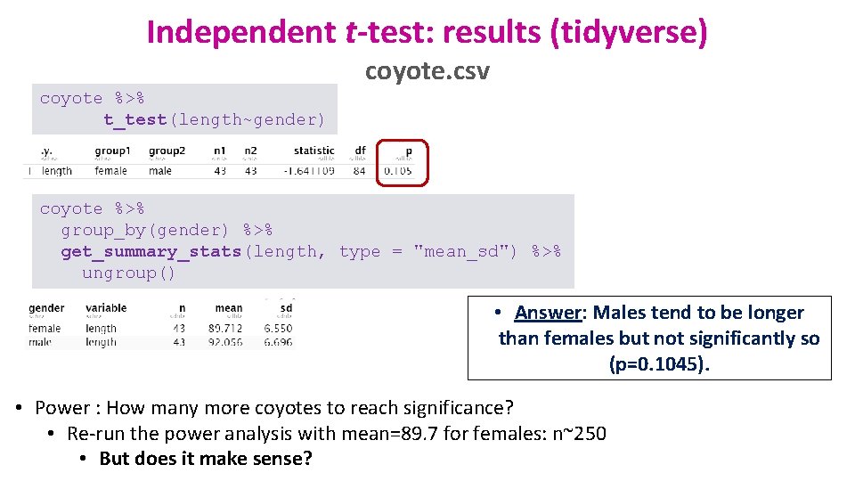
Independent t-test: results (tidyverse) coyote. csv coyote %>% t_test(length~gender) coyote %>% group_by(gender) %>% get_summary_stats(length, type = "mean_sd") %>% ungroup() • Answer: Males tend to be longer than females but not significantly so (p=0. 1045). • Power : How many more coyotes to reach significance? • Re-run the power analysis with mean=89. 7 for females: n~250 • But does it make sense?

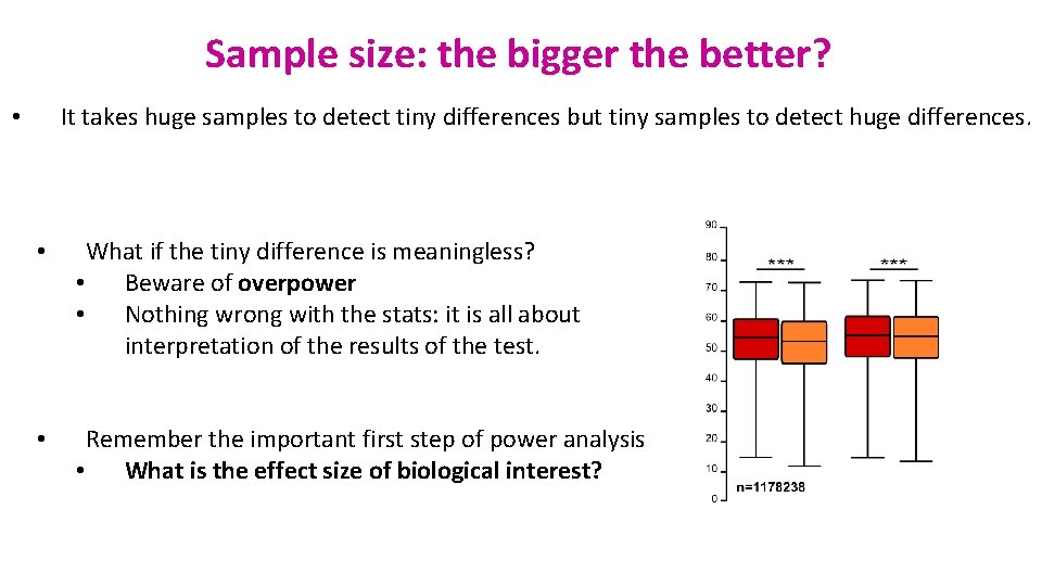
Sample size: the bigger the better? It takes huge samples to detect tiny differences but tiny samples to detect huge differences. • • What if the tiny difference is meaningless? • Beware of overpower • Nothing wrong with the stats: it is all about interpretation of the results of the test. • Remember the important first step of power analysis • What is the effect size of biological interest?

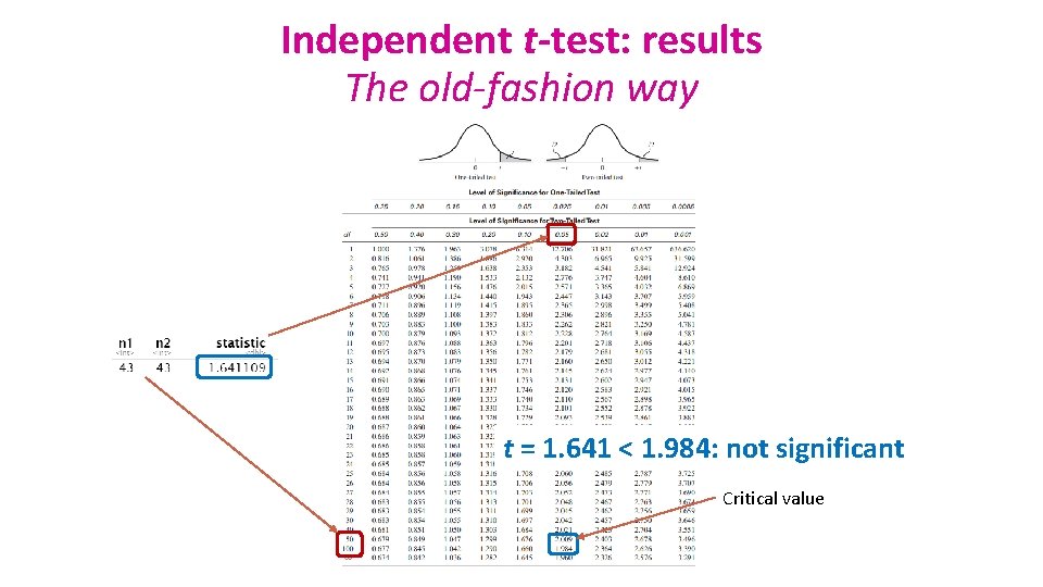
Independent t-test: results The old-fashion way t = 1. 641 < 1. 984: not significant Critical value

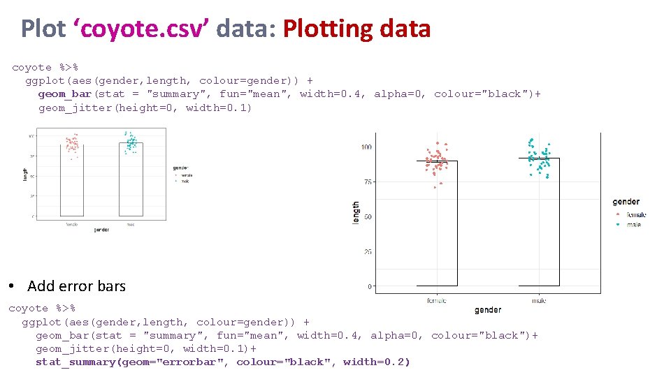
Plot ‘coyote. csv’ data: Plotting data coyote %>% ggplot(aes(gender, length, colour=gender)) + geom_bar(stat = "summary", fun="mean", width=0. 4, alpha=0, colour="black")+ geom_jitter(height=0, width=0. 1) • Add error bars coyote %>% ggplot(aes(gender, length, colour=gender)) + geom_bar(stat = "summary", fun="mean", width=0. 4, alpha=0, colour="black")+ geom_jitter(height=0, width=0. 1)+ stat_summary(geom="errorbar", colour="black", width=0. 2)

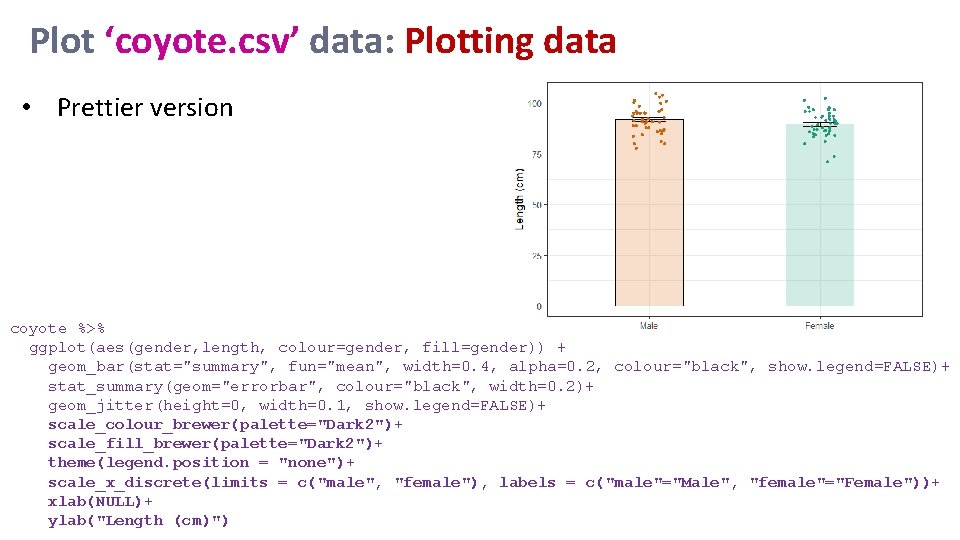
Plot ‘coyote. csv’ data: Plotting data • Prettier version coyote %>% ggplot(aes(gender, length, colour=gender, fill=gender)) + geom_bar(stat="summary", fun="mean", width=0. 4, alpha=0. 2, colour="black", show. legend=FALSE)+ stat_summary(geom="errorbar", colour="black", width=0. 2)+ geom_jitter(height=0, width=0. 1, show. legend=FALSE)+ scale_colour_brewer(palette="Dark 2")+ scale_fill_brewer(palette="Dark 2")+ theme(legend. position = "none")+ scale_x_discrete(limits = c("male", "female"), labels = c("male"="Male", "female"="Female"))+ xlab(NULL)+ ylab("Length (cm)")

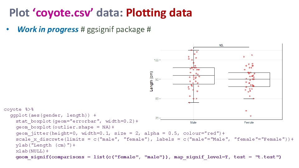
Plot ‘coyote. csv’ data: Plotting data • Work in progress # ggsignif package # coyote %>% ggplot(aes(gender, length)) + stat_boxplot(geom="errorbar", width=0. 2)+ geom_boxplot(outlier. shape = NA)+ geom_jitter(height=0, width=0. 1, size = 2, alpha = 0. 5, colour="red")+ scale_x_discrete(limits = c("male", "female"), labels = c("male"="Male", "female"="Female"))+ ylab("Length (cm)")+ xlab(NULL)+ geom_signif(comparisons = list(c("female", "male")), map_signif_level=T, test = "t. test")

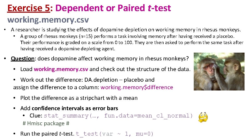
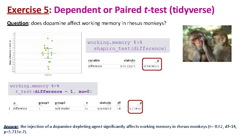
Exercise 5: Dependent or Paired t-test working. memory. csv • A researcher is studying the effects of dopamine depletion on working memory in rhesus monkeys. • A group of rhesus monkeys (n=15) performs a task involving memory after having received a placebo. Their performance is graded on a scale from 0 to 100. They are then asked to perform the same task after having received a dopamine depleting agent. • Question: does dopamine affect working memory in rhesus monkeys? • Load working. memory. csv and check out the structure of the data. • Work out the difference: DA. depletion – placebo and assign the difference to a column: working. memory$difference • Plot the difference as a stripchart with a mean • Add confidence intervals as error bars • Clue: stat_summary(…, fun. data=mean_cl_normal) # Hmisc package # • Run the paired t-test. t_test(var ~ 1, mu=0)

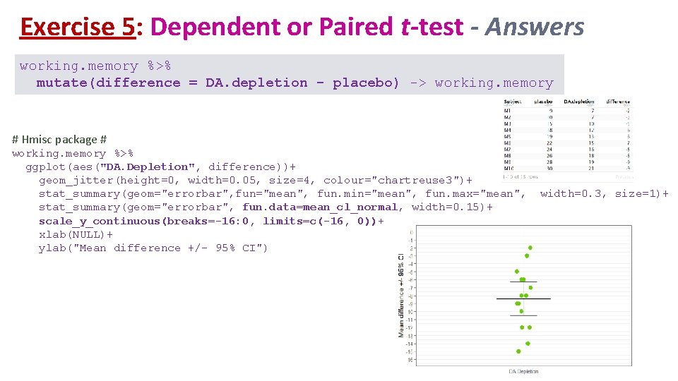
Exercise 5: Dependent or Paired t-test - Answers working. memory %>% mutate(difference = DA. depletion - placebo) -> working. memory # Hmisc package # working. memory %>% ggplot(aes("DA. Depletion", difference))+ geom_jitter(height=0, width=0. 05, size=4, colour="chartreuse 3")+ stat_summary(geom="errorbar", fun="mean", fun. min="mean", fun. max="mean", stat_summary(geom="errorbar", fun. data=mean_cl_normal, width=0. 15)+ scale_y_continuous(breaks=-16: 0, limits=c(-16, 0))+ xlab(NULL)+ ylab("Mean difference +/- 95% CI") width=0. 3, size=1)+

Exercise 5: Dependent or Paired t-test (tidyverse) Question: does dopamine affect working memory in rhesus monkeys? working. memory %>% shapiro_test(difference) working. memory %>% t_test(difference ~ 1, mu=0) Answer: the injection of a dopamine-depleting agent significantly affects working memory in rhesus monkeys (t=-8. 62, df=14, p=5. 715 e-7).

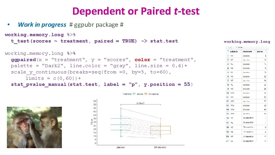
Dependent or Paired t-test • Work in progress # ggpubr package # working. memory. long %>% t_test(scores ~ treatment, paired = TRUE) -> stat. test working. memory. long %>% ggpaired(x = "treatment", y = "scores", color = "treatment", palette = "Dark 2", line. color = "gray", line. size = 0. 4)+ scale_y_continuous(breaks=seq(from =0, by=5, to=60), limits = c(0, 60))+ stat_pvalue_manual(stat. test, label = "p", y. position = 55) working. memory. long