Analysis of quantitative data Describe Infer Honours Project
Analysis of quantitative data: Describe & Infer Honours Project 4900 2010 Gavin T L Brown, Ph. D
Scientific Research Processes 1. 2. 3. 4. 5. 6. Pose significant questions that can be investigated empirically Link research to relevant theory Use methods that permit direct investigation of the question Provide coherent and explicit chain of reasoning Replicate & generalise across studies Disclose research to encourage professional scrutiny & critique
What do we want to know? � Can we use these data? ◦ Types of variables ◦ Issues—missing data; cleaning & checking; normality � What have we got in each variable? ◦ Descriptive statistics: N, M, SD ◦ Cross-tabulations � Are things the same? Inferential statistics ◦ relative to chance (statistical significance) p value and appropriate tests t-test, F-test ◦ Scale of differences (practical significance) effect size,
Structure of quantitative data � Matrix; spreadsheet ◦ Rows, columns, cells � Rows=cases, participants, all info about 1 person � Columns=variables (the things we are interested in on which cases VARY or differ) � Cells=intersection of variables x case (contains values for case) � Data entry in SPSS in DATA VIEW
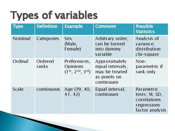
Types of variables Type Definition Example Comment Possible Statistics Nominal Categories Sex (Male, Female) Arbitrary order; can be turned into dummy variable Analysis of variance; distribution chi-square Ordinal Ordered ranks Preferences, Opinions (1 st, 2 nd, 3 rd) Approximately equal intervals; may be treated as points on continuum Nonparametric if rank only Scale continuous Age (39, 40, 41, 42) Equal interval, continuum Parametric tests; M, SD, correlations regressions factor analysis
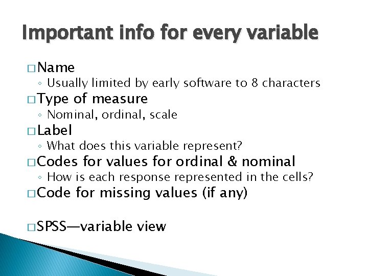
Important info for every variable � Name ◦ Usually limited by early software to 8 characters � Type of measure ◦ Nominal, ordinal, scale � Label ◦ What does this variable represent? � Codes for values for ordinal & nominal ◦ How is each response represented in the cells? � Code for missing values (if any) � SPSS—variable view
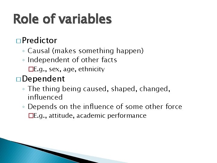
Role of variables � Predictor ◦ Causal (makes something happen) ◦ Independent of other facts �E. g. , sex, age, ethnicity � Dependent ◦ The thing being caused, shaped, changed, influenced ◦ Depends on the influence of some other force �E. g. , attitude, academic performance
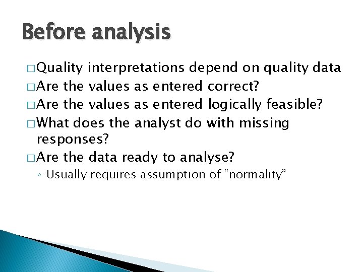
Before analysis � Quality interpretations depend on quality data � Are the values as entered correct? � Are the values as entered logically feasible? � What does the analyst do with missing responses? � Are the data ready to analyse? ◦ Usually requires assumption of “normality”
Basic Description � Is the centre and spread of each variable more or less normal?
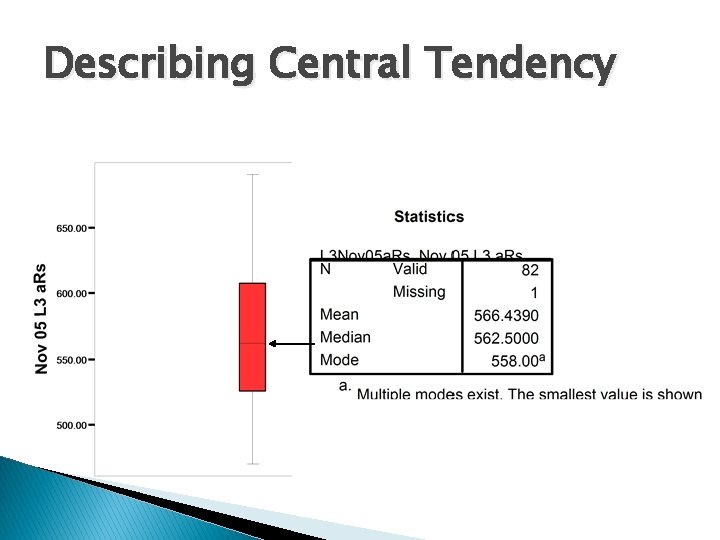
Describing Central Tendency � Where is the middle? ◦ Mean (M)—arithmetic average of all scores �Compulsory approach for continuous data ◦ Mode—most frequent score; �good approach for categorical data ◦ Median—score for person at mid-point of distribution (50 th percentile) �Good for both continuous and categorical data
Describing Central Tendency
Describing Spread � Variance—an indication of how closely the central tendency score represents the true values ◦ Large variance means mean/mode/median does not represent all people well � Standard Deviation ◦ The value that summarises the distribution of scores around the centre point
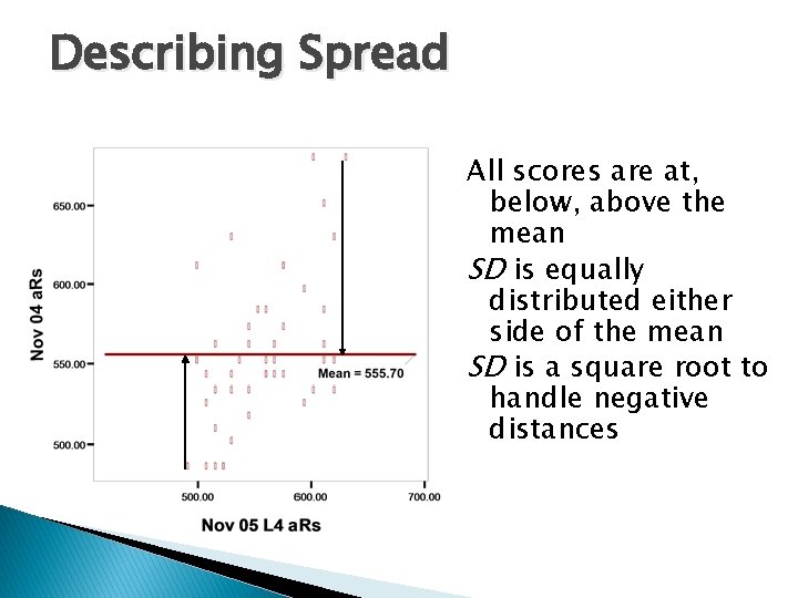
Describing Spread All scores are at, below, above the mean SD is equally distributed either side of the mean SD is a square root to handle negative distances
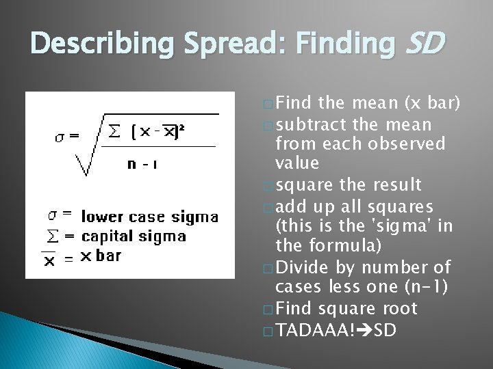
Describing Spread: Finding SD � Find the mean (x bar) � subtract the mean from each observed value � square the result � add up all squares (this is the 'sigma' in the formula) � Divide by number of cases less one (n-1) � Find square root � TADAAA! SD
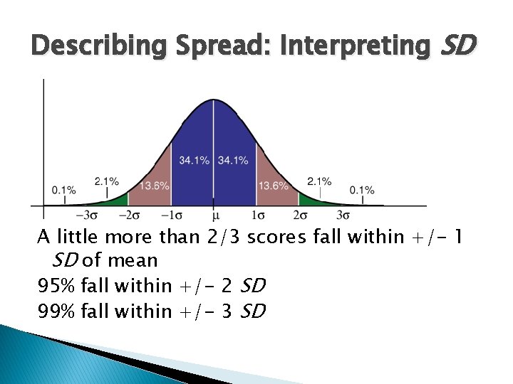
Describing Spread: Interpreting SD A little more than 2/3 scores fall within +/- 1 SD of mean 95% fall within +/- 2 SD 99% fall within +/- 3 SD
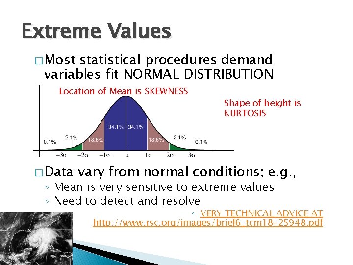
Extreme Values � Most statistical procedures demand variables fit NORMAL DISTRIBUTION Location of Mean is SKEWNESS � Data Shape of height is KURTOSIS vary from normal conditions; e. g. , ◦ Mean is very sensitive to extreme values ◦ Need to detect and resolve ◦ VERY TECHNICAL ADVICE AT http: //www. rsc. org/images/brief 6_tcm 18 -25948. pdf
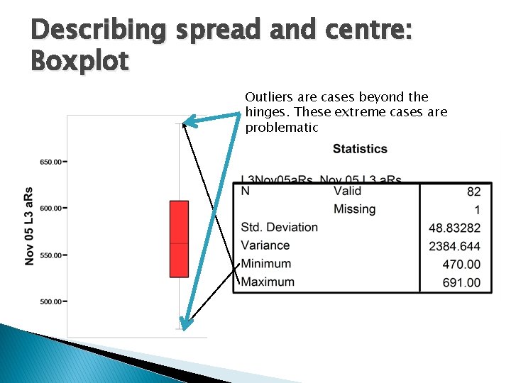
Describing spread and centre: Boxplot Outliers are cases beyond the hinges. These extreme cases are problematic
Extreme Values � Normality detection ◦ Check kurtosis (height) & skewness (location of centre) �(+/-3. 0 no problem)+in some cases as high as 7. 00 is ok � Outlier detection ◦ Check boxplot displays for people with extreme values per variable �Possibly remove or adjust using a trimming technique �Winsorise: 90% Winsorised mean sets the bottom 5% to the 5 th percentile, the top 5% to the 95 th percentile, and then averages the data.
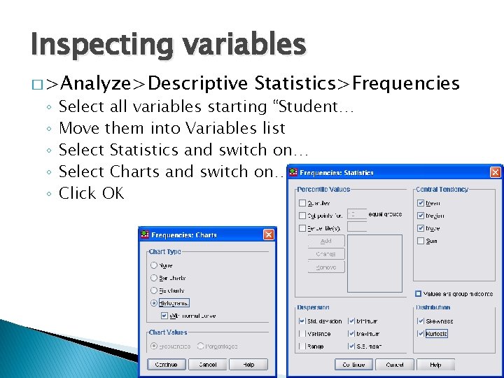
Inspecting variables � >Analyze>Descriptive ◦ ◦ ◦ Statistics>Frequencies Select all variables starting “Student… Move them into Variables list Select Statistics and switch on… Select Charts and switch on… Click OK
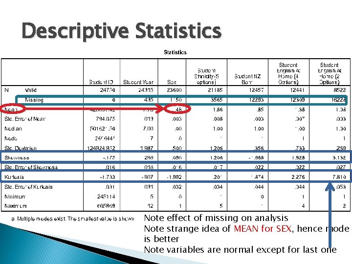
Descriptive Statistics Note effect of missing on analysis Note strange idea of MEAN for SEX, hence mode is better Note variables are normal except for last one
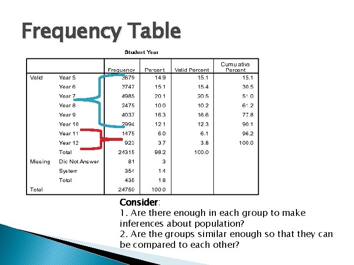
Frequency Table Consider: 1. Are there enough in each group to make inferences about population? 2. Are the groups similar enough so that they can be compared to each other?
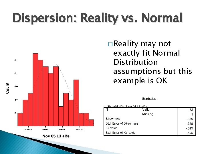
Dispersion: Reality vs. Normal � Reality may not exactly fit Normal Distribution assumptions but this example is OK
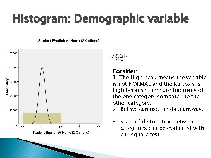
Histogram: Demographic variable Consider: 1. The High peak means the variable is not NORMAL and the Kurtosis is high because there are too many of the one category compared to the other category. 2. But we can use the data anyway. 3. Scale of distribution between categories can be evaluated with chi-square test
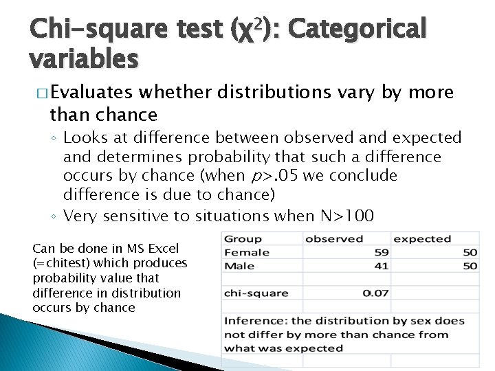
Chi-square test (χ2): Categorical variables � Evaluates whether distributions vary by more than chance ◦ Looks at difference between observed and expected and determines probability that such a difference occurs by chance (when p>. 05 we conclude difference is due to chance) ◦ Very sensitive to situations when N>100 Can be done in MS Excel (=chitest) which produces probability value that difference in distribution occurs by chance
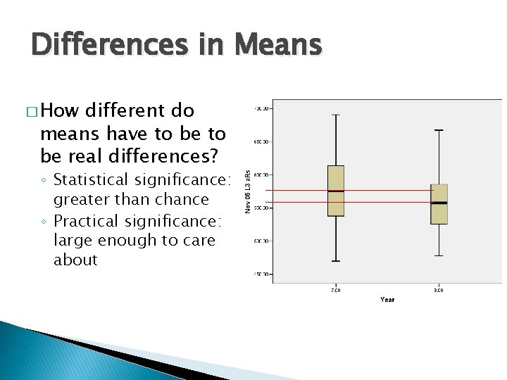
Differences in Means � How different do means have to be real differences? ◦ Statistical significance: greater than chance ◦ Practical significance: large enough to care about
Means are rarely identical � Chance eliminated by statistical inferential tests of difference of means ◦ t-test: difference of means adjusted by degrees of freedom; if p<. 05, then means differ by more than chance ◦ F-test: difference of means adjusted by variance in scores within each group (BETTER); if p<. 05, then means differ by more than chance
Student’s t-test � Observed Value 1 (+/- 2 std errors) minus Observed Value 2 (+/- 2 std errors) � Compare result to critical values of that result appearing by chance given number of cases � good for small sample n<30 � Uses ◦ Compare sub-group to overall mean ◦ Compare two different groups � Prone to interpretive error if multiple tests conducted
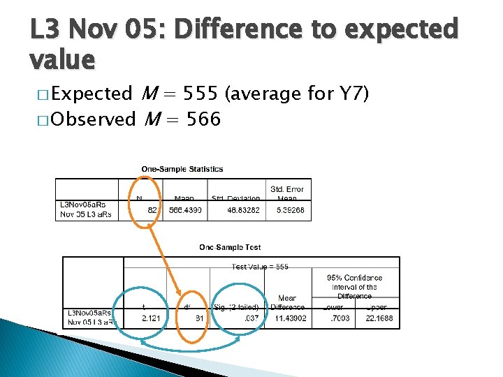
L 3 Nov 05: Difference to expected value M = 555 (average for Y 7) � Observed M = 566 � Expected
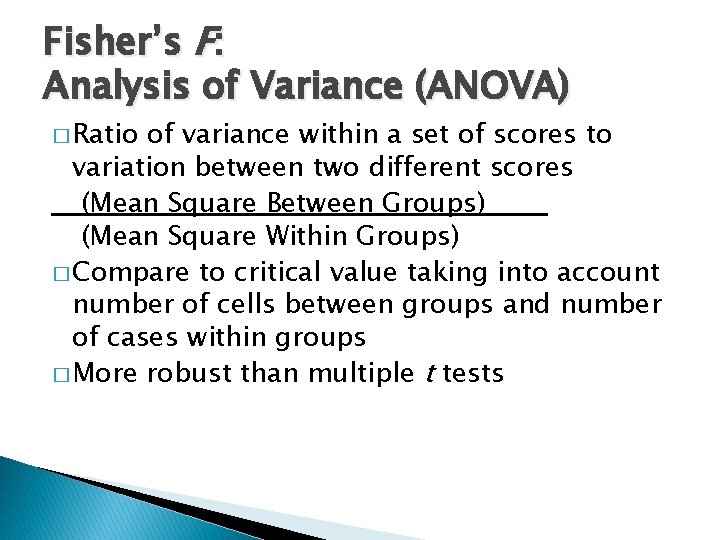
Fisher’s F: Analysis of Variance (ANOVA) � Ratio of variance within a set of scores to variation between two different scores (Mean Square Between Groups) (Mean Square Within Groups) � Compare to critical value taking into account number of cells between groups and number of cases within groups � More robust than multiple t tests
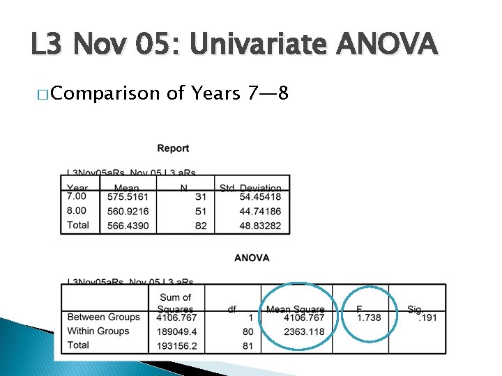
L 3 Nov 05: Univariate ANOVA � Comparison of Years 7— 8
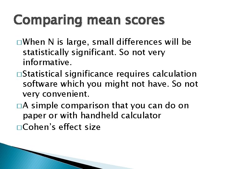
Comparing mean scores � When N is large, small differences will be statistically significant. So not very informative. � Statistical significance requires calculation software which you might not have. So not very convenient. � A simple comparison that you can do on paper or with handheld calculator � Cohen’s effect size
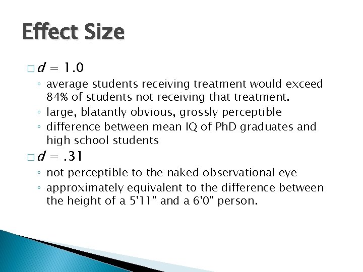
Effect Size �d = 1. 0 �d =. 31 ◦ average students receiving treatment would exceed 84% of students not receiving that treatment. ◦ large, blatantly obvious, grossly perceptible ◦ difference between mean IQ of Ph. D graduates and high school students ◦ not perceptible to the naked observational eye ◦ approximately equivalent to the difference between the height of a 5'11" and a 6'0" person.
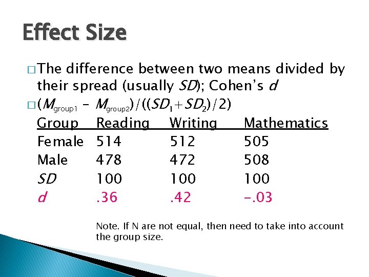
Effect Size � The difference between two means divided by their spread (usually SD); Cohen’s d � (Mgroup 1 – Mgroup 2)/((SD 1+SD 2)/2) Group Reading Writing Mathematics Female 514 512 505 Male 478 472 508 SD 100 100 d. 36. 42 -. 03 Note. If N are not equal, then need to take into account the group size.
Differences in means � Effects need to be medium with moderate N to be statistically significant � Effect size and inferential statistics lead to similar conclusions � Need to report both inferential and practical significance when comparing means
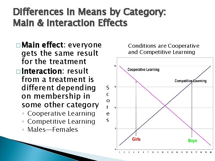
Differences in Means by Category: Main & Interaction Effects � Main effect: everyone gets the same result for the treatment � Interaction: result from a treatment is different depending on membership in some other category ◦ Cooperative Learning ◦ Competitive Learning ◦ Males—Females Conditions are Cooperative and Competitive Learning S c o r e s
Correlations �A correlation is a measure of degree to which two variables behave in a similar manner; it’s the linear relationship ◦ Positive = both go up together ◦ Negative = one goes up, the other goes down ◦ Zero = means no meaningful pattern in relationship of variables � Variables are RARELY perfectly correlated in social science—small correlations are normal
Measurement: Correlations �A measure of how similar 2 or more traits are in how they increase & decrease ◦ As human height increases there is a strong tendency for weight to increase ◦ As human age increases there is a strong tendency for weight and height to increase ◦ As human age increases there is a strong tendency for personal wealth to increase ◦ As human age increases there is a strong tendency for more books to be published
Logical errors with correlations � Possible to assume correlation equals causation ◦ My weight & income are correlated ◦ my increasing weight is causing my income to increase (get fat makes you rich!) � Possible to assume a correlation equals real connection rather than chance ◦ My age and number of books published are positively correlated ◦ But this is purely coincidental
Meaning of Correlation Values � Square of correlation = percentage of variance explained Interpretation � Small sizes � Medium � Large Correlation ranges . 01 to. 20 Variance explained up to 4% likely to be chance unless very large sample . 20 to. 50 to. 99 4 --25% 25 --98%
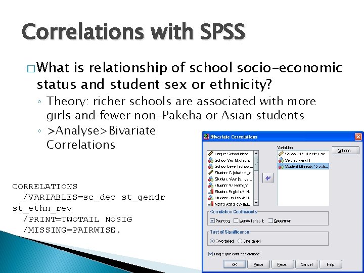
Correlations with SPSS � What is relationship of school socio-economic status and student sex or ethnicity? ◦ Theory: richer schools are associated with more girls and fewer non-Pakeha or Asian students ◦ >Analyse>Bivariate Correlations CORRELATIONS /VARIABLES=sc_dec st_gendr st_ethn_rev /PRINT=TWOTAIL NOSIG /MISSING=PAIRWISE.
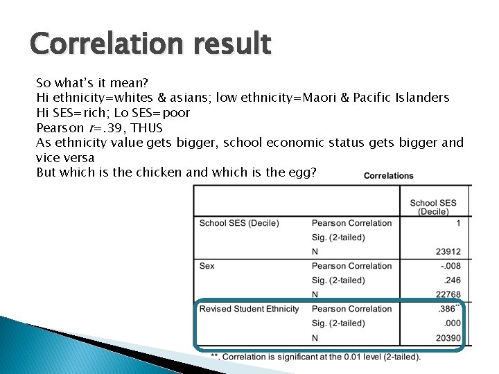
Correlation result So what’s it mean? Hi ethnicity=whites & asians; low ethnicity=Maori & Pacific Islanders Hi SES=rich; Lo SES=poor Pearson r=. 39, THUS As ethnicity value gets bigger, school economic status gets bigger and vice versa But which is the chicken and which is the egg?
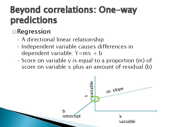
Beyond correlations: One-way predictions � Regression Y variable ◦ A directional linear relationship ◦ Independent variable causes differences in dependent variable: Y=mx + b ◦ Score on variable y is equal to a proportion (m) of score on variable x plus an amount of residual (b) b intercept pe o l s : m X variable
Regression � The amount of increase (beta) in a dependent variable as a function of predictor variables � Standardise increase as a proportion of standard deviation (standardised beta [β]) ◦ Conceptually similar to an effect size ◦ Square of β indicates proportion of variance in dependent variable explained by predictor
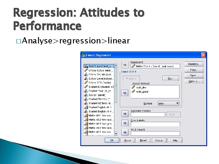
Regression: Attitudes to Performance � Analyse>regression>linear
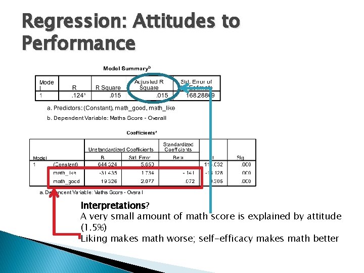
Regression: Attitudes to Performance Interpretations? A very small amount of math score is explained by attitude (1. 5%) Liking makes math worse; self-efficacy makes math better
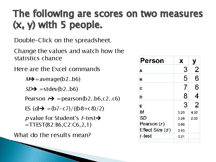
The following are scores on two measures (x, y) with 5 people. Double-Click on the spreadsheet. Change the values and watch how the statistics chance Here are the Excel commands M =average(b 2. . b 6) SD =stdev(b 2. . b 6) Pearson r =pearson(b 2. . b 6, c 2. . c 6) ES (d) =(b 7 -c 7)/((b 8+c 8)/2) p value for Student’s t-test =TTEST(B 2: B 6, C 2: C 6, 2, 1) What do the results mean?
- Slides: 46