Analysis of Oil Seeds Grain Price Volatility in

Analysis of Oil Seeds & Grain Price Volatility in India: A VEC-MVGARCH Approach A Research Proposal by Dr Alok Pandey, Ph. D. Associate Professor (Finance) IMT Ghaziabad

Background • Oilseeds and wheat grains have witnessed unprecedented volatilities and price fluctuations in the recent past. • Extreme volatility in commodity prices, particularly of food commodities, affects producers, consumers, traders, exporters & food procurement agencies of the central and state Government.

Commodities Under Study • Wheat • Selected Edible Oil seeds and Oil Wheat & Edible Oil Price Forecast World Bank. xls

Wheat Price Volatility • Who plays the biggest role in pushing the global wheat prices now? • It is India. • Following India’s plan to buy more wheat for buffer stock, the commodity’s prices soared across the world with the World Food Programme (WFP) expressing concern over the impact of dwindling stocks of the cereal.

Wheat Price Volatility • After India invited tenders for an unspecified quantity of wheat from the international market, the price of wheat crossed record levels on commodity exchanges on Thursday. • As grain traders reacted to urgent tenders from grain importers and the lowest global stock levels for 25 years, the prices shot up across the globe. • India is the world’s second-largest wheat producer after China, but orders from Delhi to build up buffer stocks pushed price of a bushel climbing 30 cents to $7. 88 a bushel on the Chicago Board of Trade.

Wheat Price Volatility • In France, the price of November milling wheat also soared. • Natural calamities like droughts and floods and production shortfalls, burgeoning demand dwindling stocks also created a harvest season panic that again pushed the prices of wheat further. • Since April, it has risen 75 per cent on both sides of the Atlantic after recent tenders from Egypt and India.

Wheat Price Volatility • India last year suffered a weak harvest and entered the world market aggressively to import wheat. The International Grains Council expects India to import more than three million tonnes this year, despite an improved harvest. Analysts believe that there is growing anxiety that the country had benefited from a succession of good monsoons.

Wheat Price Volatility • The International Grain Council cut its forecast of world grain production by seven million tonnes this month to 607 million tonnes, as it assessed the impact of a wet summer in Northern Europe, weak output in Ukraine and drought in Argentina and Australia. • Chicago Board of Trade wheat Futures contract set a new all-time high this week as crop concerns roil the market again. The December contract took out last week’s previous all-time high of $7. 54.

Wheat Price Volatility • Paris wheat Futures settled just shy of their all-time high and London-based wheat Futures surpassed their previous top. More talk of Australian drought conditions and wheat crop woes there was another reason for bulls to buy.

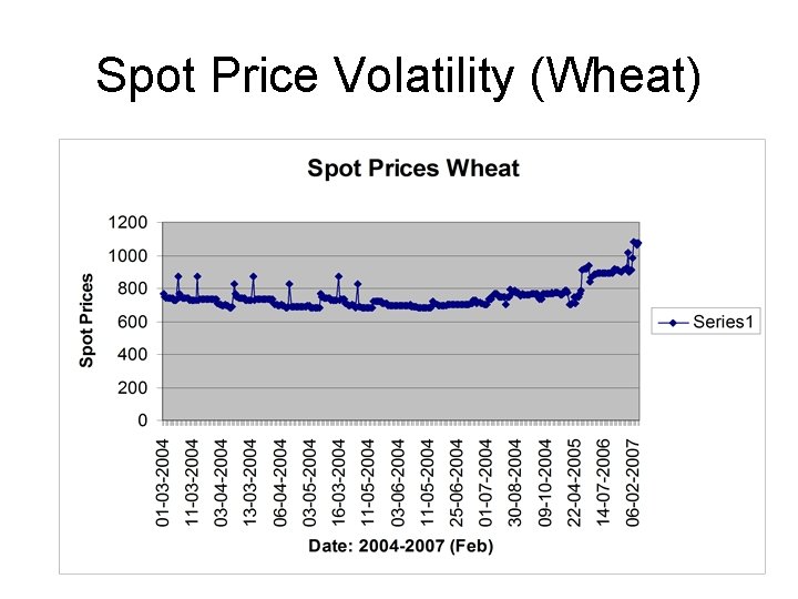
Spot Price Volatility (Wheat)

Oil & Oilseeds Caster Seed / Caster Oil Coconut Oil / Copra Cotton Seed / Cottonseed Oil Crude Palm Oil Ground Nut / Groundnut Oil Kapasia Khalli Linseed / Linseed Oil

Oil & Oilseeds Mustard Oil / Mustard Seed /Mustard Seed Oil RBD Palmolein / Refined Soy Oil Refined Sunflower Oil Rice Bran Refined Oil Safflower / Safflower Oil Sesam Oil Soy Meal /Soybean / Soyabean Oil / Sunflower Oil/ Sunflower Seed

Oil & Oil Seeds • India is the world’s fourth largest edible oil economy with 15, 000 oil mills, 689 solvent extraction units, 251 Vanaspati plants and over 1, 000 refineries employing more than one million people. • The total market size is at Rs. 600, 000 Mln. and import export trade is worth Rs. 130, 000 Mln.

Oil & Oil Seeds • India being deficient in oils has to import 40% of its consumption requirements. • With an annual consumption of about 11 mln. Tonnes, the per capita consumption is at 11. 50 kgs, which is very low compared to world average of 20 kgs. • China is currently at 17 kg.

Overview of Edible Oil Economy • Indian vegetable oil is world's fourth largest after USA, China and Brazil. • Oilseed cultivation is undertaken across the country in two seasons, in about 26 million hectares; mainly on marginal lands, dependent on monsoon rains (un-irrigated) and with low levels of input usage. • Yields are rather low at less than one ton per hectare.

Overview of Edible Oil Economy • Three oilseeds - Groundnut, Soybean and Rapeseed/ Mustard - together account for over 80 per cent of aggregate cultivated oilseeds output. • Mustard seed alone contributes Rs. 120, 000 Mln. turnover out of Rs. 600, 000 Mln. oilseed based Sector domestic turnover. • Cottonseed, Copra and other oil-bearing material too contribute to domestic vegetable oil pool

Overview of Edible Oil Economy • Currently, India accounts for 7. 0% of world oilseeds output; 7. 0% of world oil meal production; 6. 0% of world oil meal export; 6. 0% of world veg. oil production; 14% of world veg. oil import; and 10 % of the world edible oil consumption • With steady growth in population and personal income, Indian per capita consumption of edible oil has been growing steadily. • However, oilseeds output and in turn, vegetable oil production have been trailing consumption growth, necessitating imports to meet supply shortfall.

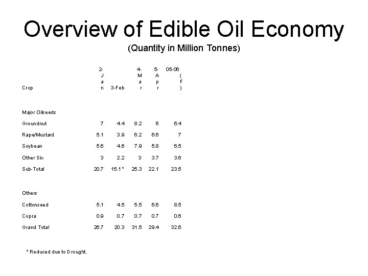
Overview of Edible Oil Economy (Quantity in Million Tonnes) 3 -Feb 4 M a r 5 A p r 7 4. 4 8. 2 6 6. 4 Rape/Mustard 5. 1 3. 9 6. 2 6. 6 7 Soybean 5. 6 4. 6 7. 9 5. 8 6. 5 Other Six 3 2. 2 3 3. 7 3. 6 Sub-Total 20. 7 15. 1 * 25. 3 22. 1 23. 5 Cottonseed 5. 1 4. 5 5. 5 6. 6 8. 5 Copra 0. 9 0. 7 0. 6 26. 7 20. 3 31. 5 29. 4 32. 6 Crop 2 J a n 05 -06 ( F ) Major Oilseeds Groundnut Others Grand Total * Reduced due to Drought.

Overview of Edible Oil Economy • 80 per cent of India's domestic oil output comes from the primary source that is nine cultivated oilseeds and two major oilbearing materials (Cottonseed and Copra). The secondary source comprises of solvent extracted oils, Rice bran oil, oils from minor and tree-borne oilseeds etc.

Market Potential • The per capita consumption of oil in India is 11. 5 kg/year is way below the world average of 18 kg. Even china is at 17 kg. By 2010 the per capita consumption of oil in India is likely to be 15. 6 kg. There is huge potential of growth. • The demand for edible oils is expected to increase from Oil Year 2004 -05 levels of 10. 9 Mln. tonnes to 12. 3 Mln. tonnes by 2006 -07 (two years). This assumes a per capita consumption increase of 4% and a population growth of 1. 9% which translates to an overall growth in demand @ 6% p. a. Based on the above assumptions, edible oil demand in the year 2015 is expected to be 21. 3 million tonnes.

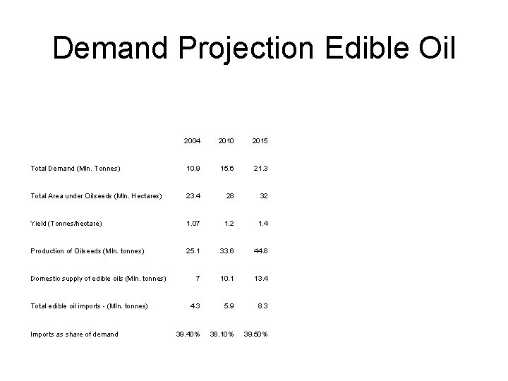
Demand Projection Edible Oil 2004 2010 2015 Total Demand (Mln. Tonnes) 10. 9 15. 6 21. 3 Total Area under Oilseeds (Mln. Hectares) 23. 4 28 32 Yield (Tonnes/hectare) 1. 07 1. 2 1. 4 Production of Oilseeds (Mln. tonnes) 25. 1 33. 6 44. 8 7 10. 1 13. 4 4. 3 5. 9 8. 3 39. 40% 38. 10% 39. 50% Domestic supply of edible oils (Mln. tonnes) Total edible oil imports - (Mln. tonnes) Imports as share of demand

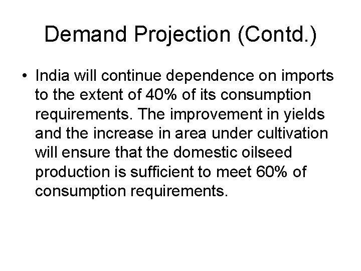
Demand Projection (Contd. ) • India will continue dependence on imports to the extent of 40% of its consumption requirements. The improvement in yields and the increase in area under cultivation will ensure that the domestic oilseed production is sufficient to meet 60% of consumption requirements.

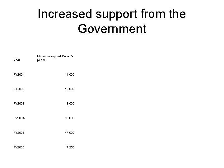
Increased support from the Government Year Minimum support Price Rs. per MT FY 2001 11, 000 FY 2002 12, 000 FY 2003 13, 000 FY 2004 16, 000 FY 2005 17, 000 FY 2006 17, 250

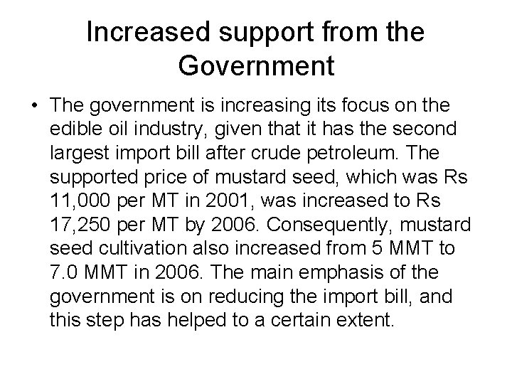
Increased support from the Government • The government is increasing its focus on the edible oil industry, given that it has the second largest import bill after crude petroleum. The supported price of mustard seed, which was Rs 11, 000 per MT in 2001, was increased to Rs 17, 250 per MT by 2006. Consequently, mustard seed cultivation also increased from 5 MMT to 7. 0 MMT in 2006. The main emphasis of the government is on reducing the import bill, and this step has helped to a certain extent.

Spot Price Volatility (Wheat)

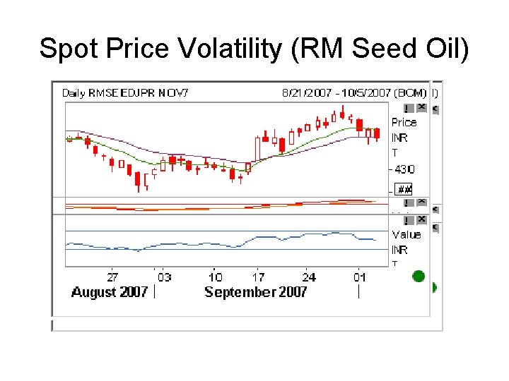
Spot Price Volatility (RM Seed Oil)

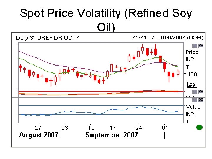
Spot Price Volatility (Refined Soy Oil)

Objectives • This paper proposes a multivariate vector error -correction generalized autoregressive conditional heteroscedasticity model to investigate the effect of oilseeds and wheat grain prices in neighbouring countries of Asia on its Indian equivalents. • We propose to test whether in the long run the law of one price holds and whether in the short run the model captures the salient features of Indian commodity prices (oilseeds and wheat grain).

Objectives (Contd. ) • This model will be used to compute rolling forecasts of the conditional means, variances and covariance of the prices of oilseeds and wheat grain one year ahead. • We expect that this model will produce superior forecasts compared to those based on a commonly used methodology of an autoregressive conditional mean model where the second moments are estimated using a fixed weight moving average.

Objectives • • To measure the degree of price instability of important agricultural commodities in the major international and domestic markets. The commodities selected for the study are wheat, palm oil, groundnut oil, soybean oil and coconut oil. To Compare the patterns of variability in Asian markets and understand its implications for Indian producers and consumers.

Objectives (Contd. ) • • To examine whether the conditional mean relationship between Asian and Indian grain and oilseed prices can be characterized by a vector error correction (VEC) model. To examine how well do the one-year ahead forecasts of the conditional first and second moments from the VEC-MVGARCH model compare with those generated using the Chavas and Holt (1990) methodology and whethere is a significant difference in these forecasts using Hansen’s (2001) recently developed test of superior predictive ability (SPA).

Methodology • The research methodology broadly is based on following three steps: 1. Modeling the Mean and Volatility of Indian oilseeds and wheat grain prices using ARCH, GARCH and ARIMA models. 2. Testing the data to examine whether the conditional mean relationship between Asian (few select countries independently) and Indian oilseed and wheat grain prices can be characterized by a vector error correction (VEC) model based on short and long run theory of Law of One Price (LOP). 3. Expanding the VEC model to allow for the modeling of the time varying second moments of domestic oilseeds and grain prices using a MVGARCH model.

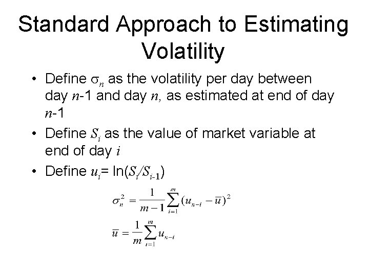
Standard Approach to Estimating Volatility • Define sn as the volatility per day between day n-1 and day n, as estimated at end of day n-1 • Define Si as the value of market variable at end of day i • Define ui= ln(Si/Si-1)

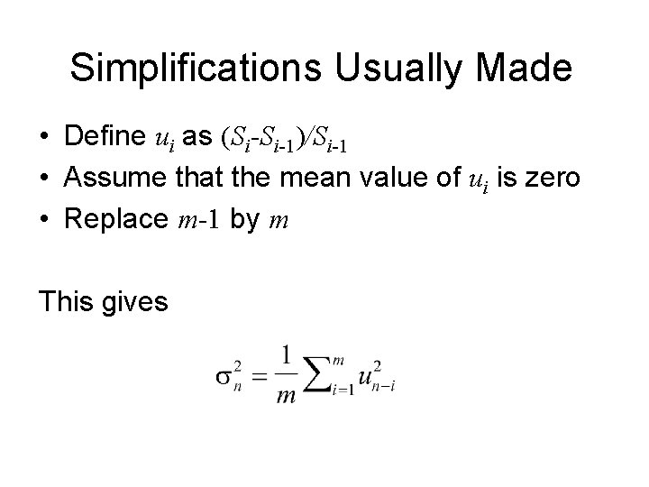
Simplifications Usually Made • Define ui as (Si-Si-1)/Si-1 • Assume that the mean value of ui is zero • Replace m-1 by m This gives

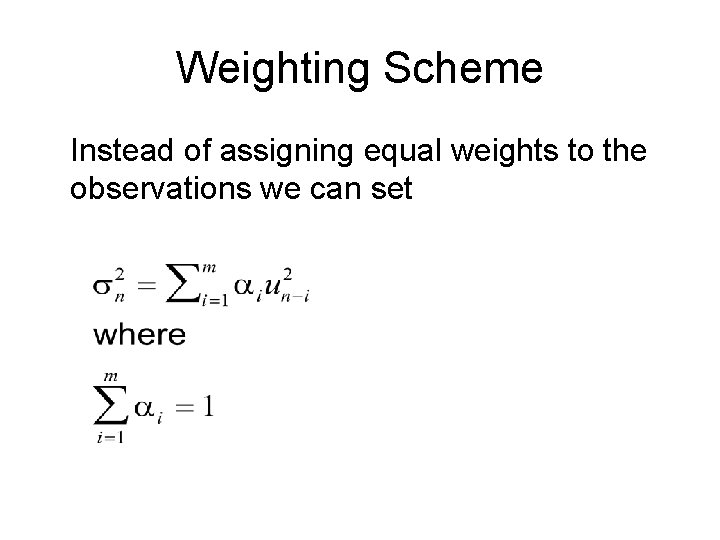
Weighting Scheme Instead of assigning equal weights to the observations we can set

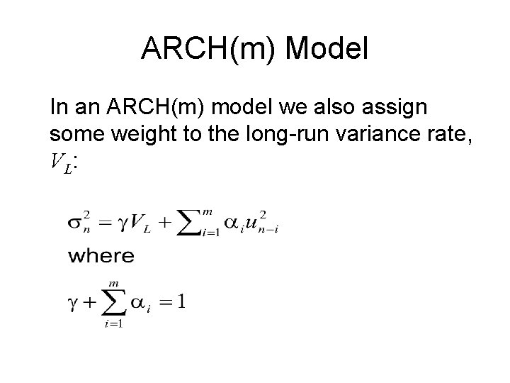
ARCH(m) Model In an ARCH(m) model we also assign some weight to the long-run variance rate, V L:

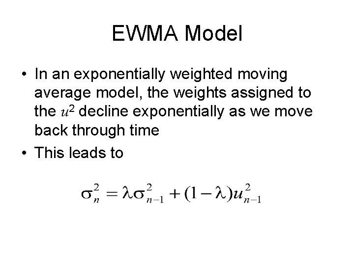
EWMA Model • In an exponentially weighted moving average model, the weights assigned to the u 2 decline exponentially as we move back through time • This leads to

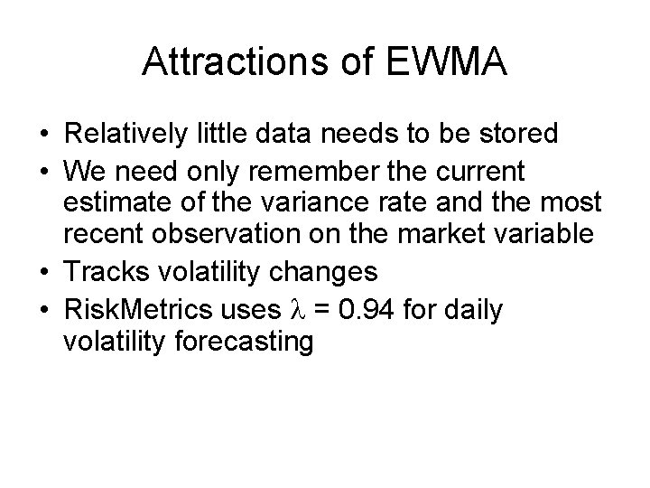
Attractions of EWMA • Relatively little data needs to be stored • We need only remember the current estimate of the variance rate and the most recent observation on the market variable • Tracks volatility changes • Risk. Metrics uses l = 0. 94 for daily volatility forecasting

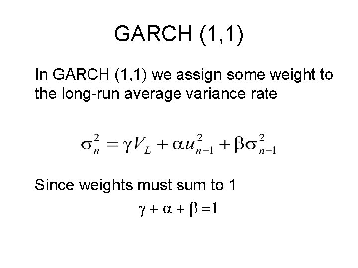
GARCH (1, 1) In GARCH (1, 1) we assign some weight to the long-run average variance rate Since weights must sum to 1 g + a + b =1

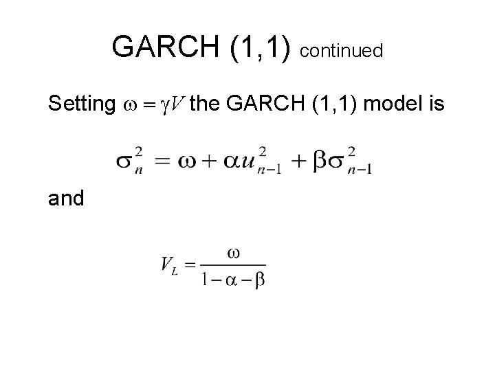
GARCH (1, 1) continued Setting w = g. V the GARCH (1, 1) model is and

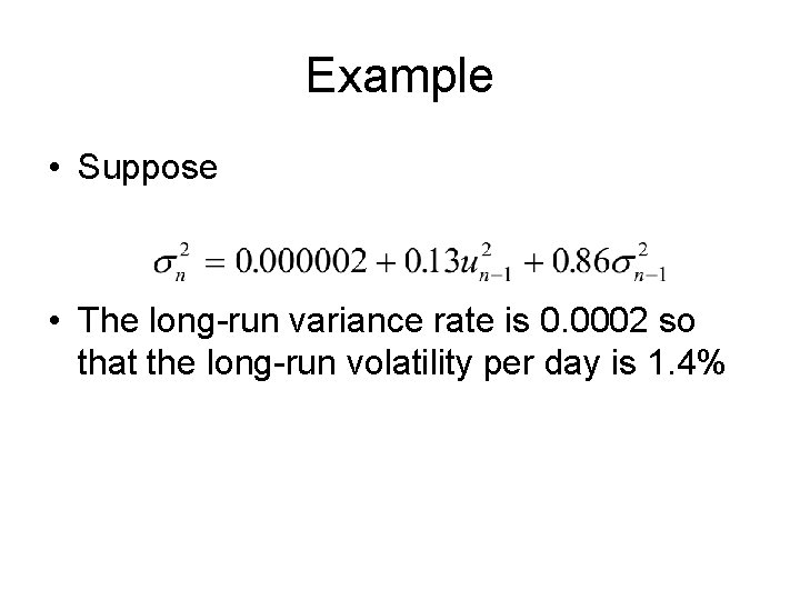
Example • Suppose • The long-run variance rate is 0. 0002 so that the long-run volatility per day is 1. 4%

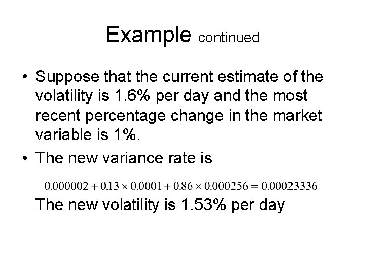
Example continued • Suppose that the current estimate of the volatility is 1. 6% per day and the most recent percentage change in the market variable is 1%. • The new variance rate is The new volatility is 1. 53% per day

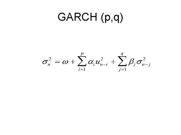
GARCH (p, q)

Maximum Likelihood Methods • In maximum likelihood methods we choose parameters that maximize the likelihood of the observations occurring

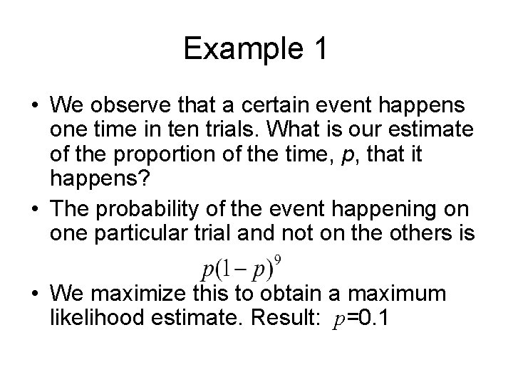
Example 1 • We observe that a certain event happens one time in ten trials. What is our estimate of the proportion of the time, p, that it happens? • The probability of the event happening on one particular trial and not on the others is • We maximize this to obtain a maximum likelihood estimate. Result: p=0. 1

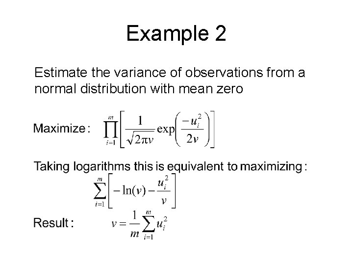
Example 2 Estimate the variance of observations from a normal distribution with mean zero

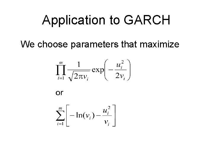
Application to GARCH We choose parameters that maximize

Variance Targeting • One way of implementing GARCH(1, 1) that increases stability is by using variance targeting • We set the long-run average volatility equal to the sample variance • Only two other parameters then have to be estimated

How Good is the Model? • The Ljung-Box statistic tests for autocorrelation • We compare the autocorrelation of the ui 2 with the autocorrelation of the ui 2/si 2

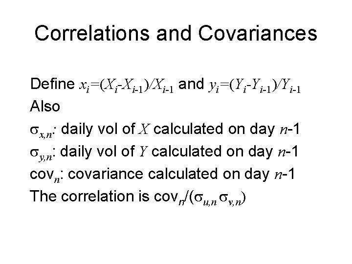
Correlations and Covariances Define xi=(Xi-Xi-1)/Xi-1 and yi=(Yi-Yi-1)/Yi-1 Also sx, n: daily vol of X calculated on day n-1 sy, n: daily vol of Y calculated on day n-1 covn: covariance calculated on day n-1 The correlation is covn/(su, n sv, n)

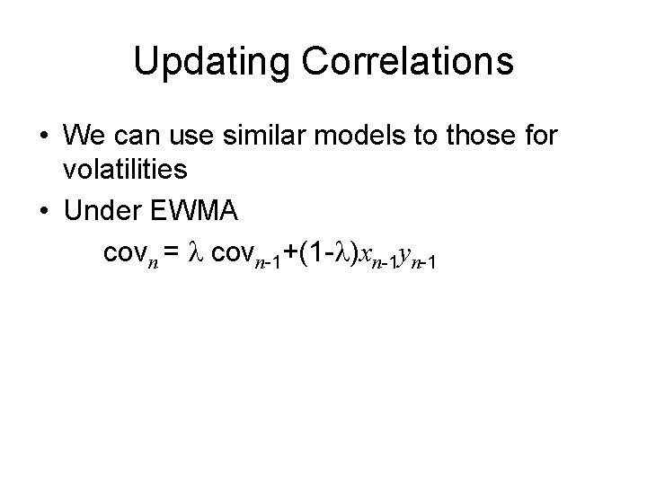
Updating Correlations • We can use similar models to those for volatilities • Under EWMA covn = l covn-1+(1 -l)xn-1 yn-1

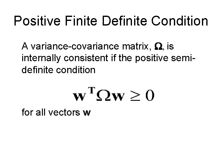
Positive Finite Definite Condition A variance-covariance matrix, W, is internally consistent if the positive semidefinite condition for all vectors w

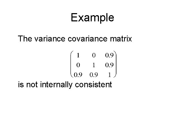
Example The variance covariance matrix is not internally consistent

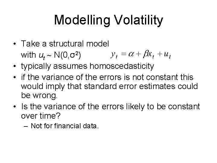
Modelling Volatility • Take a structural model with ut N(0, σ2) • typically assumes homoscedasticity • if the variance of the errors is not constant this would imply that standard error estimates could be wrong. • Is the variance of the errors likely to be constant over time? – Not for financial data.

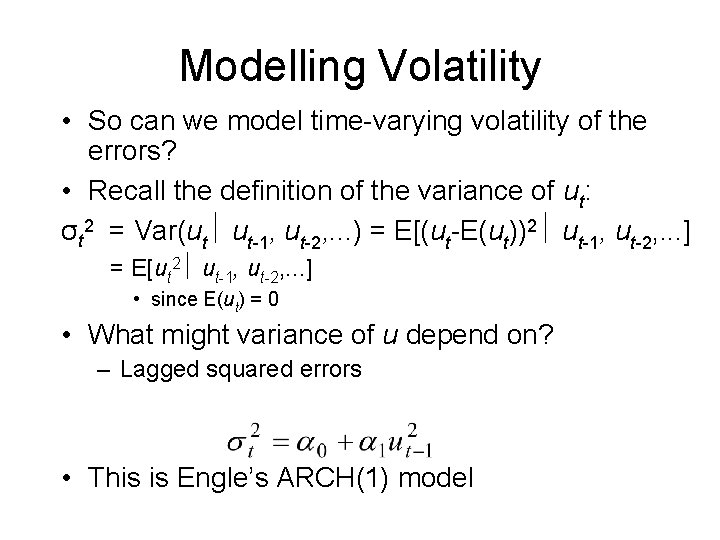
Modelling Volatility • So can we model time-varying volatility of the errors? • Recall the definition of the variance of ut: σt 2 = Var(ut ut-1, ut-2, . . . ) = E[(ut-E(ut))2 ut-1, ut-2, . . . ] = E[ut 2 ut-1, ut-2, . . . ] • since E(ut) = 0 • What might variance of u depend on? – Lagged squared errors • This is Engle’s ARCH(1) model

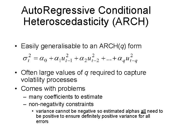
Auto. Regressive Conditional Heteroscedasticity (ARCH) • Easily generalisable to an ARCH(q) form • Often large values of q required to capture volatility processes • Comes with problems – many coefficients to estimate – non-negativity constraints • variance cannot be negative so estimated alphas all need to be positive to ensure definitely positive variance for all errors

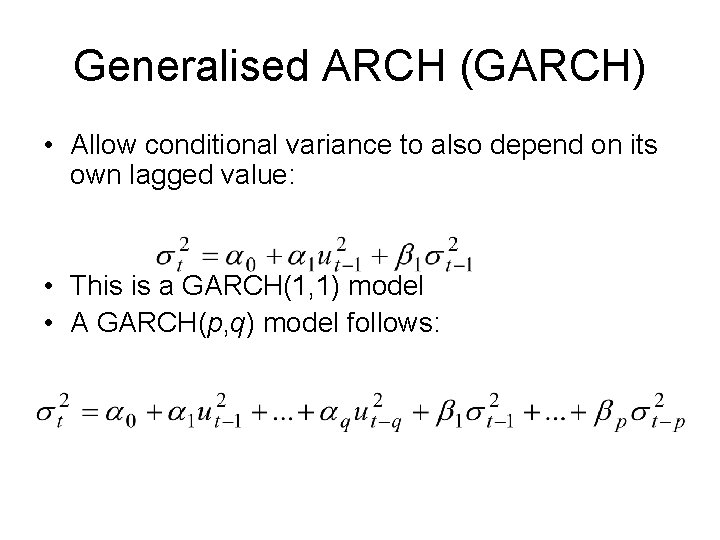
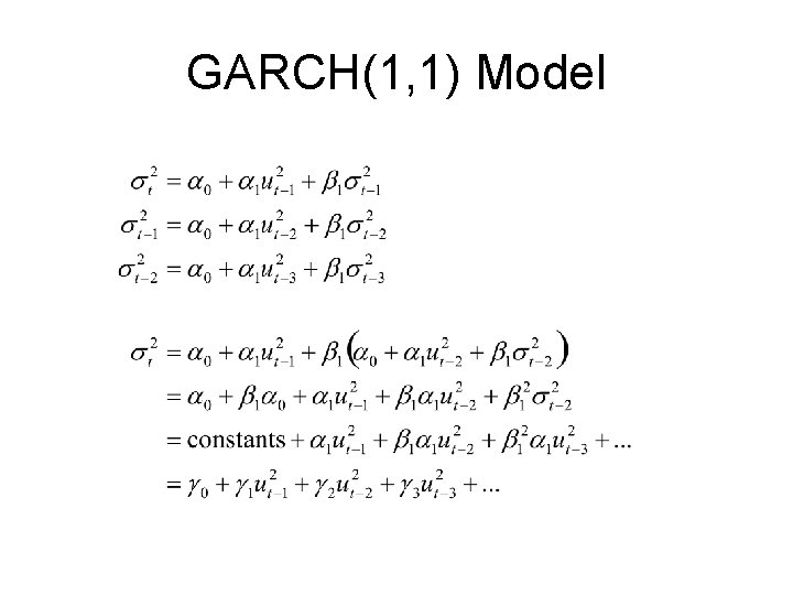
Generalised ARCH (GARCH) • Allow conditional variance to also depend on its own lagged value: • This is a GARCH(1, 1) model • A GARCH(p, q) model follows:

GARCH(1, 1) Model

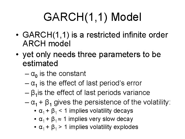
GARCH(1, 1) Model • GARCH(1, 1) is a restricted infinite order ARCH model • yet only needs three parameters to be estimated – α 0 is the constant – α 1 is the effect of last period’s error – β 1 is the effect of last periods variance – α 1 + β 1 gives the persistence of the volatility: • α 1 + β 1 < 1 implies volatility decays • α 1 + β 1 1 implies very slow decay • α 1 + β 1 > 1 implies volatility explodes

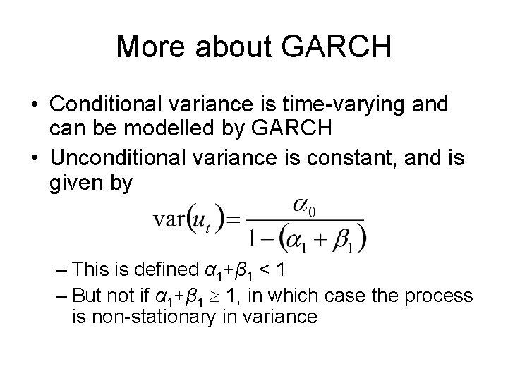
More about GARCH • Conditional variance is time-varying and can be modelled by GARCH • Unconditional variance is constant, and is given by – This is defined α 1+β 1 < 1 – But not if α 1+β 1 1, in which case the process is non-stationary in variance

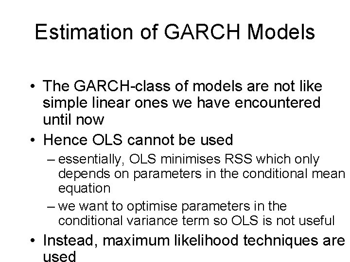
Estimation of GARCH Models • The GARCH-class of models are not like simple linear ones we have encountered until now • Hence OLS cannot be used – essentially, OLS minimises RSS which only depends on parameters in the conditional mean equation – we want to optimise parameters in the conditional variance term so OLS is not useful • Instead, maximum likelihood techniques are

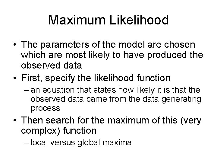
Maximum Likelihood • The parameters of the model are chosen which are most likely to have produced the observed data • First, specify the likelihood function – an equation that states how likely it is that the observed data came from the data generating process • Then search for the maximum of this (very complex) function – local versus global maxima

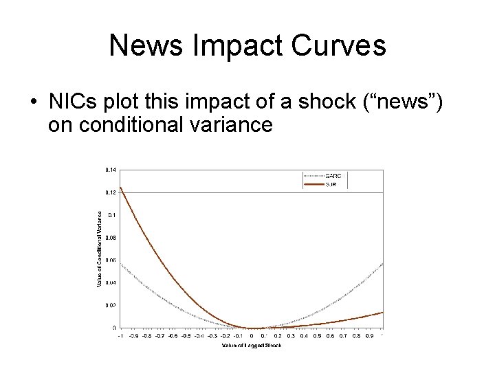
Extensions • Asymmetric GARCH – In a basic GARCH model, the conditional variance is determined by last period’s variance and last period’s error squared – So a positive error has the same effect on variance as a negative error – This need not always be a good assumption

Leverage Effects • Suppose there is a negative shock to the equity return of a company • This increases the leverage of the firm (equity value down, debt unchanged) • So the risk of the equity has risen • A positive shock to the equity reduces leverage and has a negative impact on risk (other things ignored) • A negative error has a larger effect than a positive error

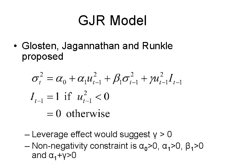
GJR Model • Glosten, Jagannathan and Runkle proposed – Leverage effect would suggest γ > 0 – Non-negativity constraint is α 0>0, α 1>0, β 1>0 and α 1+γ>0

News Impact Curves • NICs plot this impact of a shock (“news”) on conditional variance

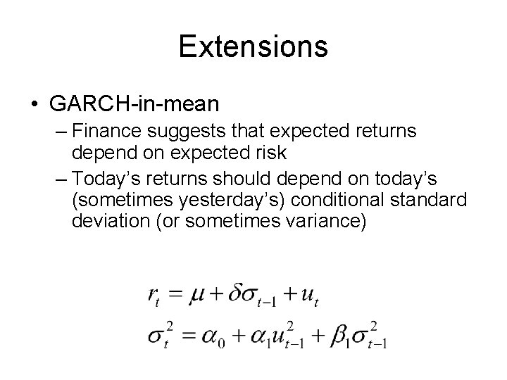
Extensions • GARCH-in-mean – Finance suggests that expected returns depend on expected risk – Today’s returns should depend on today’s (sometimes yesterday’s) conditional standard deviation (or sometimes variance)

GARCH-in-Mean • An increase in risk, given by the conditional standard deviation leads to a rise in the mean return • The value of δ gives the increase in returns needed to compensate for a give increase in risk • So is a measure of risk aversion

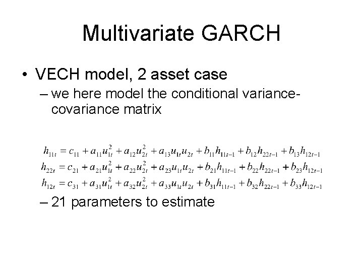
Extensions • Multivariate GARCH – Univariate GARCH models capture the evolution of conditional variances – Multivariate GARCH models also capture movements in conditional covariances – These look quite complicated and use a lot of matrix algebra – But are really quite simple (honest)

Multivariate GARCH • VECH model, 2 asset case – we here model the conditional variancecovariance matrix – 21 parameters to estimate

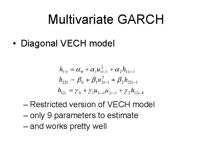
Multivariate GARCH • Diagonal VECH model – Restricted version of VECH model – only 9 parameters to estimate – and works pretty well

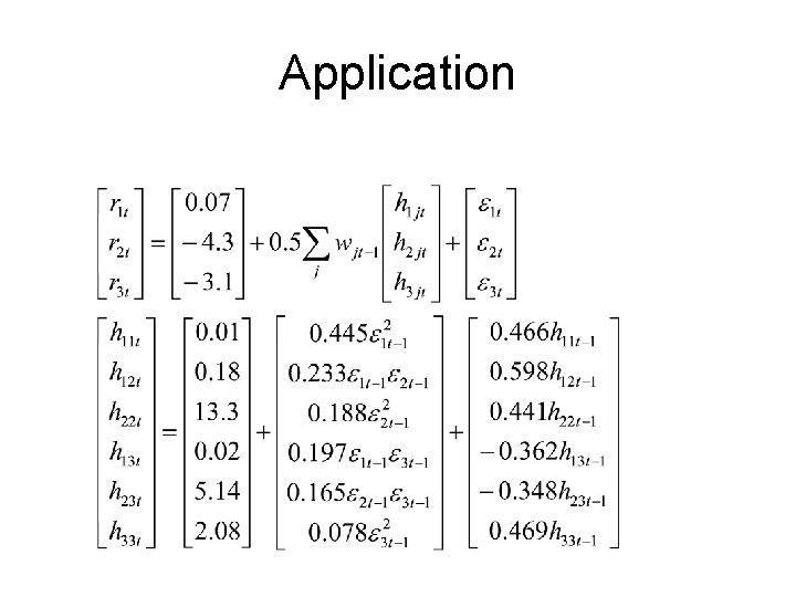
Application • Bollerslev, Engleand Wooldridge (1988) • Multivariate diagonal VECH GARCH-inmean model – US T-bills (asset 1) – US T-bonds (asset 2) – US equities (asset 3) – 1959 Q 1 -1984 Q 2

Application

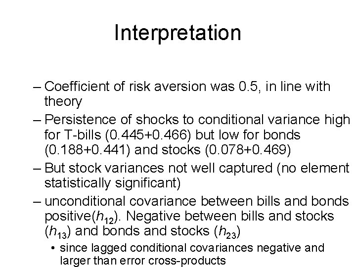
Interpretation – Coefficient of risk aversion was 0. 5, in line with theory – Persistence of shocks to conditional variance high for T-bills (0. 445+0. 466) but low for bonds (0. 188+0. 441) and stocks (0. 078+0. 469) – But stock variances not well captured (no element statistically significant) – unconditional covariance between bills and bonds positive(h 12). Negative between bills and stocks (h 13) and bonds and stocks (h 23) • since lagged conditional covariances negative and larger than error cross-products

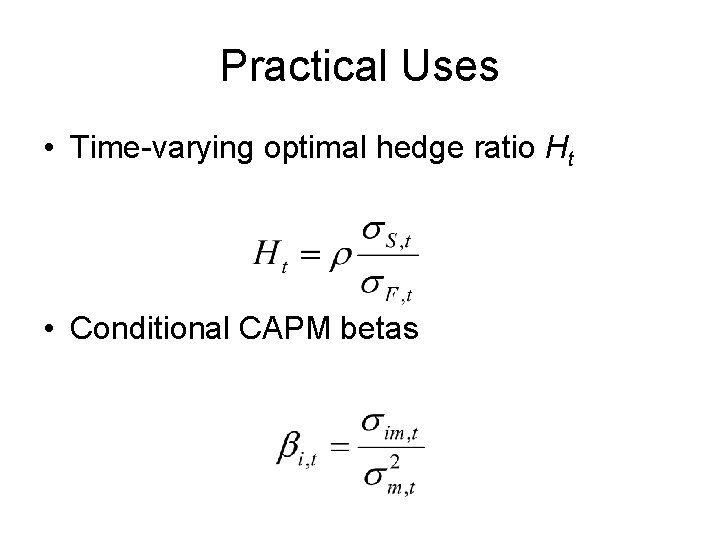
Practical Uses • Time-varying optimal hedge ratio Ht • Conditional CAPM betas

VEC Models

The Chavas Holt Methodology (1990)

Hansen’s Test of SPA (2001)

The MV GARCH Model

Sources of Data

Limitations of the Study