Analysis of multivariate time series In this presentation

 Vector Auto. Regressive (VAR) Multivariate time series Vector")


 instead of VAR(1)? Companion matrix")


, p = 1, type = 'none') fit 2 =")


![EG test § Matlab: [h, pvalue, stat, c. Value, reg] = egcitest(Y_new, 'test', 't](https://slidetodoc.com/presentation_image_h/7a492b540dd5d30be3818a0fb906935a/image-19.jpg "EG test § Matlab: [h, pvalue, stat, c. Value, reg] = egcitest(Y_new, 'test', 't")


")


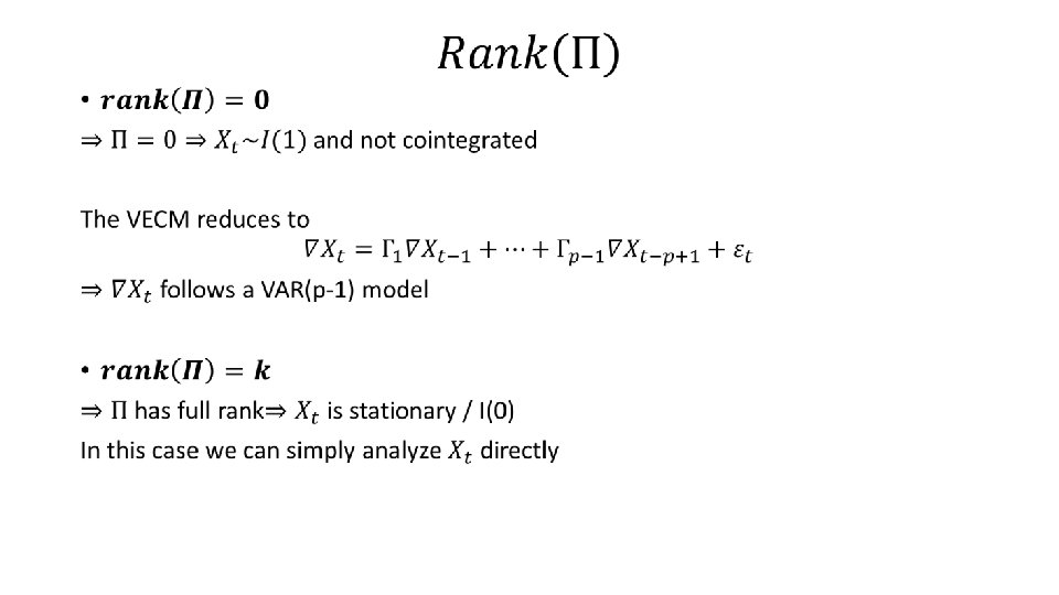
 • The drawback of Engle Granger approach: it can only identify")


 VECM (Johansen) VAR Structural VAR ARDL (ARX) Spurious")


; est. Spec =")

 Spurious")
 ~ diff(x)) Residuals: Min")
 - Univariate*/ proc VARMAX data=simul; model y z = x")
 ARDL (ARX)")
 series*/ proc reg data=simul; model dz = dx/noint;")
 series Spurious")

 ARDL (ARX)")
, Y(: , 3)) Spurious %% Regression")
 series Spurious")
 VECM (Johansen)")
![R analysis Data generation ECM (E-G) VECM (Johansen) Y[i] = 0. 4918 X[i] +](https://slidetodoc.com/presentation_image_h/7a492b540dd5d30be3818a0fb906935a/image-73.jpg "R analysis Data generation ECM (E-G) VECM (Johansen) Y[i] = 0. 4918 X[i] +")
 proc AUTOREG data = simul; model y =")
 Rejection of null hypothesis indicates existence of cointegration.")
)")

![Matlab analysis Data generation ECM (E-G) Y_new = [Y(: , 2) Y(: , 1)];](https://slidetodoc.com/presentation_image_h/7a492b540dd5d30be3818a0fb906935a/image-78.jpg "Matlab analysis Data generation ECM (E-G) Y_new = [Y(: , 2) Y(: , 1)];")
![Matlab analysis VECM (Johansen) [h, pvalue, ~, ~, mles] =. . . jcitest(Y, 'Model',](https://slidetodoc.com/presentation_image_h/7a492b540dd5d30be3818a0fb906935a/image-79.jpg "Matlab analysis VECM (Johansen) [h, pvalue, ~, ~, mles] =. . . jcitest(Y, 'Model',")
. Co-integration and Error Correction:")

- Slides: 81
Analysis of multivariate time series In this presentation, we study the inter-relationships between several multivariate time series regression methods to provide guidance on when to use what method, and how to implement it in SAS, R, or Matlab.
Auto. Regressive Distributed Lag Model (ARDL) Vector Auto. Regressive (VAR) Multivariate time series Vector Error Correction Model (VECM) Error Correction Model (ECM)
Reduced form Structural form ARDL PCA interpretation Only one cointegration relation § Engle Granger test > one cointegration relation § VECM and Johansen test
Reduced form Structural form ARDL PCA interpretation Only one cointegration relation § Engle Granger test > one cointegration relation § VECM and Johansen test
Reduced form of VAR
Reduced form Structural form ARDL PCA interpretation Only one cointegration relation § Engle Granger test > one cointegration relation § VECM and Johansen test
Structural form of VAR
Fitting function of ARDL/ARX: § Matlab: Spec = vgxset('n', 1, 'n. AR', 1, 'n. X', 1, 'Constant', false); est. Spec = vgxvarx(Spec, Y(: , 2), num 2 cell(Y(: , 1)), []); § R Univariate: fit = arima(y, c(1, 0, 0), xreg = x) § R Multivariate: fit = VAR(cbind(y, z), p = 1, type = 'none', exogen = x) § SAS: proc VARMAX; model y = x / p=1 noint;
More than two variables
What if VAR(p) instead of VAR(1)? Companion matrix
Reduced form Structural form ARDL PCA interpretation Only one cointegration relation § Engle Granger test > one cointegration relation § VECM and Johansen test
Reduced form Structural form ARDL PCA interpretation Only one cointegration relation § Engle Granger test > one cointegration relation § VECM and Johansen test
fit = VAR(cbind(x, y), p = 1, type = 'none') fit 2 = SVAR(fit, Amat = matrix(c(1, 0, NA, 1), 2, 2))
Reduced form Structural form ARDL Engle Granger test PCA interpretation Only one cointegration relation § Engle Granger test > one cointegration relation § VECM and Johansen test
They shared Nobel Memorial Prize in Economic Sciences in 2003 for the methods of ARCH (Engle), and Co-integration (Granger) respectively. Robert F. Engle (born in 1942) American economist, currently teaches at New York University, Stern School of Business Clive Granger (1934 – 2009) British economist, taught at University of Nottinghan in Britain & University of California, San Diego in US
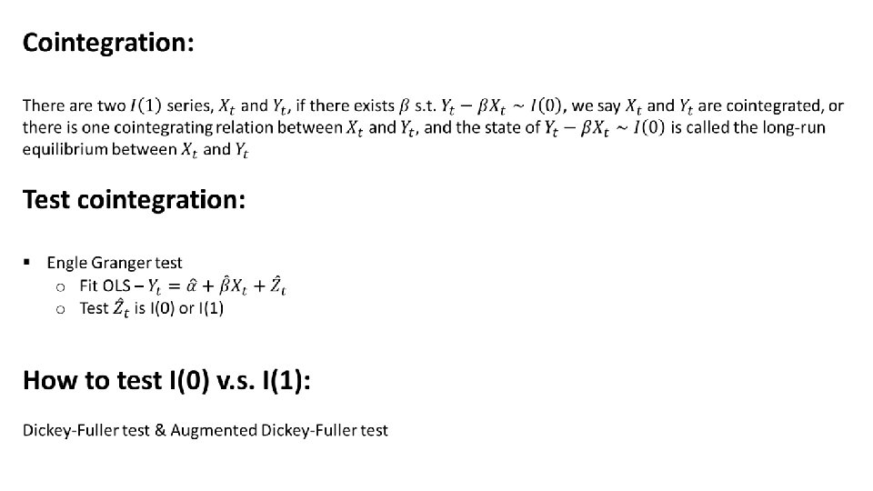
Dickey Fuller test § If there’s no drift or linear trend § To capture the nonzero mean & linear trend
Augmented Dickey Fuller test How to choose # of lags?
EG test § Matlab: [h, pvalue, stat, c. Value, reg] = egcitest(Y_new, 'test', 't 2', 'creg', 'nc'); § R: fit 5 = egcm(x, y) § SAS: proc AUTOREG; model y = x/ nlag=1 stationarity =(adf=1);
Reduced form Structural form ARDL PCA interpretation Only one cointegration relation § Engle Granger test > one cointegration relation § VECM and Johansen test
Reduced form Structural form ARDL PCA interpretation Only one cointegration relation § Engle Granger test > one cointegration relation § VECM and Johansen test
An example of cointegration
Error Correction Model (ECM)
How to fit ECM model?
Reduced form Structural form ARDL PCA interpretation Only one cointegration relation § Engle Granger test works > one cointegration relation § VECM and Johansen test
Reduced form Structural form ARDL PCA interpretation Only one cointegration relation § Engle Granger test > one cointegration relation § VECM and Johansen test
VECM for Cointegration Johansen Approach Tingjun Ruan
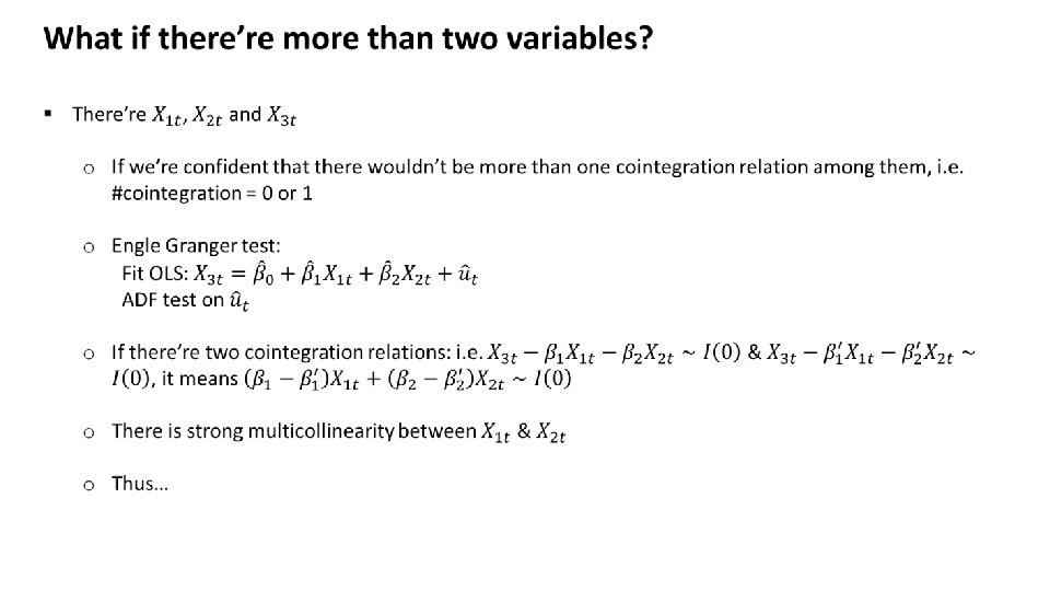
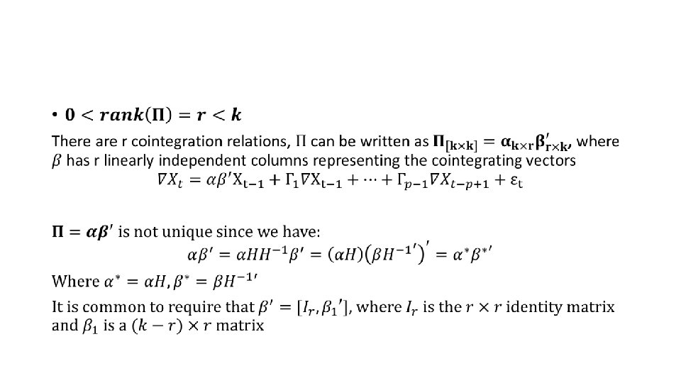
Johansen Methodology (1988) • The drawback of Engle Granger approach: it can only identify a single equilibrium relationship among the variables. If we have more than two variables in the model, then there is a possibility of having more than one cointegration relationships • Johansen (1988) proposed a framework of estimating and testing of vector error correction model (VECM) based on vector auto regressive (VAR) equations with which we can find out how many cointegrating relationships exist among variables • Johansen VECM is more general for testing multiple cointegrating relationships when there are more than two variables. • For k variables, we can have up to k-1 cointegrations
Danish Statistician and Econometrician, who is known for his research in time series analysis, in particular theory of cointegration in collaboration with Katarina Juselius. He is currently a professor at the Department of Econometrics, University of Copenhagen. Soren Johansen (born in 1939 Denmark)
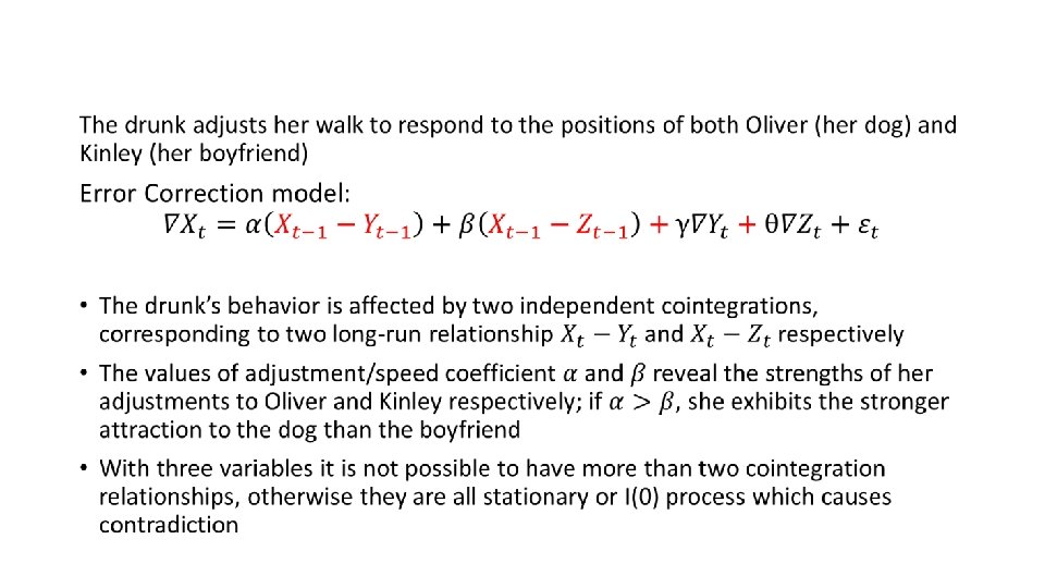
Multiple Cointegration Example - A Drunk, Her Dog and A boyfriend •
VECM •
VECM •
Determine the Number of Cointegration •
Johansen’s Trace Statistic •
Johansen’s Maximum Eigenvalue Statistic •
• The asymptotic null distribution of both tests are not Chi-square but instead a complicated function of Brownian motion and the critical values of the test statistics are non-standard • Critical values for both statistics are provided by Johansen and Juselius (1990)
Maximum Likelihood Estimation of Cointegrated VECM •
Maximum likelihood estimation •
Functions of fitting VECM and Johansen test § Matlab Johansen Procedure : [h, pvalue, ~, ~, mles] = jcitest(Y, 'Model', 'H 2', 'lags', 1, 'display', 'params') § Matlab VECM to VAR : VAR = vectovar(‘VEC’, {A 0 A 1}, ’C’, C) fit = ca. jo(cbind(x, y, z), ecdet = 'none', K = 2, spec = 'transitory') § R Johansen Procedure: fit 2 = vec 2 var(fit, r = 1) § R VECM to VAR: § SAS Johansen Procedure : proc VARMAX; model x y z / p=1 noint cointtest=(johansen=(TYPE=TRACE)) ecm = (rank=1) print = (iarr estimates); run;
Reduced form Structural form ARDL PCA interpretation Only one cointegration relation § Engle Granger test > one cointegration relation § VECM and Johansen test
Linear decomposition of cointegration Ruofeng Wen
The key of time series regression: Trend
a full-rank linear transform
So what is co-integration?
a full-rank linear transform residuals Take difference of everything and then VAR
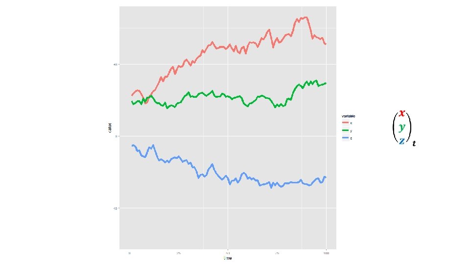
Data Simulation
independent Data generation ECM (E-G) VECM (Johansen) VAR Structural VAR ARDL (ARX) Spurious
R analysis Data generation
R analysis VAR Structural VAR
R analysis VAR Estimation Results: ============= Estimation results for equation x: ================= x = x. l 1 + y. l 1 + z. l 1 VAR Estimate Std. Error t value Pr(>|t|) x. l 1 0. 844866 0. 019799 42. 672 < 2 e-16 *** y. l 1 0. 297653 0. 039232 7. 587 7. 5 e-14 *** z. l 1 -0. 007070 0. 005301 -1. 334 0. 183 --Estimation results for equation y: ================= y = x. l 1 + y. l 1 + z. l 1 Estimate Std. Error t value Pr(>|t|) x. l 1 0. 164695 0. 012687 12. 98 <2 e-16 *** y. l 1 0. 665679 0. 025140 26. 48 <2 e-16 *** z. l 1 -0. 003465 0. 003397 -1. 02 0. 308 --Estimation results for equation z: ================= z = x. l 1 + y. l 1 + z. l 1 Estimate Std. Error t value Pr(>|t|) x. l 1 -0. 030157 0. 014928 -2. 020 0. 0436 * y. l 1 0. 050833 0. 029581 1. 718 0. 0860. z. l 1 0. 992239 0. 003997 248. 271 <2 e-16 *** ---
R analysis Warning message: In SVAR(fit 3, Amat = t(matrix(c(1, 0, 0, NA, 1, 0, 0, 0, 1), 3, Convergence not achieved after 10000 iterations. SVAR Estimation Results: ============ Estimated A matrix: x y z x 1. 0 0 0 y -0. 9 1 0 z 0. 0 0 1 Structural VAR :
SAS analysis /* Vector Autoregressive*/ proc VARMAX data=simul; model x y z / p=1 noint; run; VAR specify the order of VAR to be 1 since a VAR(1) is fitted here ; Ø p=1: Ø noint: it indicates an intercept is not included in the model.
SAS analysis output VAR
Matlab analysis Spec = vgxset('n', 3, 'n. AR', 1, 'Constant', false); est. Spec = vgxvarx(Spec, Y); vgxdisp(est. Spec) Ø vgxset: set VARMAX model specification parameters; VAR Ø ('n', 3, 'n. AR', 1, 'Constant', false): a 3 -dimensional VAR(1) with no intercept is fitted; Ø vgxvarx: estimate the VAR parameters; Ø vgxdisp: display the fitted model parameters and statistics.
Matlab analysis output VAR
R analysis ARDL (ARX) Spurious
R analysis VAR Estimation Results: ============= Call: lm(formula = diff(z) ~ diff(x)) Residuals: Min 1 Q -6. 1030 -1. 0757 Median 0. 0537 3 Q 1. 0641 Max 5. 0542 Coefficients: Estimate Std. Error t value Pr(>|t|) (Intercept) 0. 018583 0. 052993 0. 351 0. 726 diff(x) -0. 002451 0. 023256 -0. 105 0. 916 --Call: lm(formula = z ~ x) Residuals: Min 1 Q -33. 145 -11. 049 Median 3. 621 3 Q 10. 396 Estimation results for equation y: ================= y = y. l 1 + z. l 1 + exo 1 Estimate Std. Error t value Pr(>|t|) y. l 1 0. 616969 0. 022942 26. 893 <2 e-16 *** z. l 1 -0. 002243 0. 003259 -0. 688 0. 492 exo 1 0. 190141 0. 011582 16. 418 <2 e-16 *** --- ARDL (ARX) Spurious Max 27. 518 Coefficients: Estimate Std. Error t value Pr(>|t|) (Intercept) 3. 45272 0. 84049 4. 108 4. 32 e-05 *** x -0. 67996 0. 02298 -29. 588 < 2 e-16 *** ---
SAS analysis /* ARDL(ARX) - Univariate*/ proc VARMAX data=simul; model y z = x / p=1 noint; run; ARDL (ARX) /* ARDL(ARX) - Multivariate */ proc VARMAX data=simul; model y = x / p=1 noint; run; Ø y z = x : Ø p=1: a VAR includes time series Y&Z with X as a exogenous variable is fitted; order of the VAR model, “xlag= “ if you want to include lags of X in the model.
SAS analysis output ARDL(ARX) ARDL (ARX)
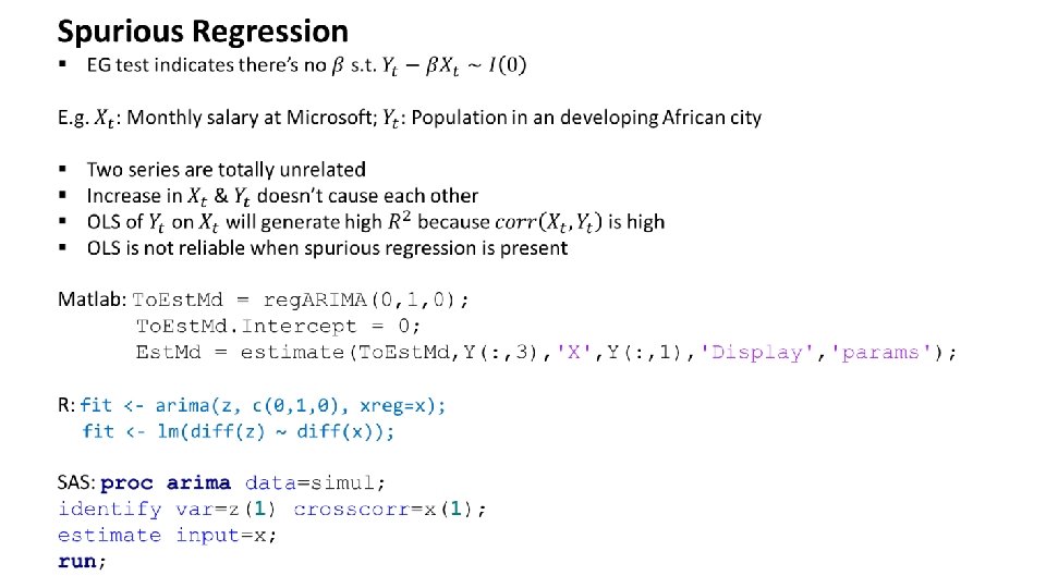
SAS analysis /*Regression of two I(1) series*/ proc reg data=simul; model dz = dx/noint; run; OR proc arima data=simul; identify var=z(1) crosscorr=x(1) ; estimate input=x noint; run; /*Spurious Regression*/ proc reg data=simul; model z = x; run; Spurious Ø var=z(1): time series z is modeled as response, the first order diffence of z is taken; Ø crosscorr=x(1): x is crosscorrelated with z and the first order difference of x is included in the model; Ø estimate input=x: specify x is the input time series, and x must be listed in crosscorr=; Ø Here Proc arima did the same fit as taking the first order difference of the two I(1) time series and then conduct OLS fit on them.
SAS analysis output Spurious Regression of two I(1) series Spurious
Matlab analysis %% ARDL multivariate Spec = vgxset('n', 2, 'n. AR', 1, 'n. X', 2, 'Constant', false); xx = cellfun(@(x) [x, 0; 0, x], . . . num 2 cell(Y(: , 1)), 'Uniform. Output', false); est. Spec = vgxvarx(Spec, Y(: , 2: 3), xx, []); vgxdisp(est. Spec) ARDL (ARX) %% ARDL univariate Spec = vgxset('n', 1, 'n. AR', 1, 'n. X', 1, 'Constant', false); est. Spec = vgxvarx(Spec, Y(: , 2), num 2 cell(Y(: , 1)), []); vgxdisp(est. Spec) Ø When fit a ARDL with two response variable, we need to specify the number of exogenous variables to be 2 via ('n. X', 2) in vgxset although we only have one exogenous variable. Then cellfun is used to create a an m-by-1 cell (m is the number of observations) to specify the exogenous variable, and j-th (j=1, …, m) cell contains a 2 -by-2 diagonal matrix with j-th element of exogenous variable on the diagonal. Ø vgxvarx: estimate the VAR parameters; Ø vgxdisp: display the fitted model parameters and statistics.
Matlab analysis ARDL(ARX) ARDL (ARX)
Matlab analysis %% Spurious Regression fitlm(Y(: , 1), Y(: , 3)) Spurious %% Regression of two I(1) time series To. Est. Md = reg. ARIMA(0, 1, 0); To. Est. Md. Intercept = 0; Est. Md = estimate(To. Est. Md, Y(: , 3), 'X', Y(: , 1), 'Display', 'params'); Ø reg. ARIMA: build regression model with ARIMA error. In practice, it takes first order difference of the two series first and then do the model fit; Ø estimate: estimate the parameters of the regression model. First argument specifies the type of the ARIMA model, and follows by the response data. 'X', Y(: , 1) specifies the input time series and 'Display', 'params‘ would show the fitted results; Ø fitlm: fit a linear regression model.
Matlab analysis Spurious Regression of two I(1) series Spurious
R analysis Data generation ECM (E-G) VECM (Johansen)
R analysis Data generation ECM (E-G) VECM (Johansen) Y[i] = 0. 4918 X[i] + 0. 3336 + R[i], R[i] = R[i-1] + eps[i], eps ~ N(0, 1. 5242^2) (0. 0031) (0. 7706) R[1000] = -1. 4247 (t = -0. 800) ########### # Johansen-Procedure # ########### Eigenvalues (lambda): [1] 1. 855745 e-01 8. 725927 e-03 3. 742696 e-05 0. 5221 (0. 0271) Values of test statistic and critical value of test: test 10 pct 5 pct 1 pct r <= 2 | 0. 04 6. 50 8. 18 11. 65 r <= 1 | 8. 75 12. 91 14. 90 19. 19 r = 0 | 204. 86 18. 90 21. 07 25. 75 Eigenvectors, normalised to first column: x. l 1 y. l 1 z. l 1 x. l 1 1. 000000 y. l 1 -2. 008998832 0. 8679812 1. 066943 z. l 1 -0. 001280153 1. 4539880 -1. 417780
SAS analysis Data generation ECM (E-G) proc AUTOREG data = simul; model y = x/ nlag=1 stationarity =(adf); run; Ø nlag=1 : specifies the order of the autoregressive error process or the subset of autoregressive error lags to be fitted; Ø stationarity =(adf): produces the augmented Dickey-Fuller unit root test. And if a regressor is presented, E-G test will be carried out to test the cointegration. The adf option is only available in recent SAS versions (after SAS 9. 2).
SAS analysis Data generation ECM (E-G) Rejection of null hypothesis indicates existence of cointegration.
SAS analysis proc VARMAX data=simul; model x y z / p=1 noint lagmax=1 cointtest=(johansen=(TYPE=TRACE)) ecm=(rank=1) print=(iarr estimates); run; VECM (Johansen) Ø p=1 specifies the order of the vector autoregressive process; Ø lagmax=1 specifies the maximum number of lags for which results are computed and displayed by the PRINT= option; Ø cointtest=(johansen=(TYPE=TRACE)) specifies johansen test to test for cointegration, here TYPE=TRACE prints the cointegration trace test which is the default and TYPE=MAX prints the cointegration maximum eigenvalue test; Ø ecm=(rank=1) is used to fit the VECM model after we know the number of cointegration from the johansen test, rank=1 specifies the number of cointegration is 1 in our case; Ø print=(iarr estimates) is used to print the reparameterized VAR coefficient matrices for the VCEM model via iarr. And estimates will print the coefficients estimates and the significance of the esitmeates.
SAS Output Johansen test indicates a cointegration of order 1. VECM in VAR form VECM (Johansen)
Matlab analysis Data generation ECM (E-G) Y_new = [Y(: , 2) Y(: , 1)]; [h, pvalue, stat, c. Value, reg] =. . . egcitest(Y_new, 'test', 't 2', 'creg', 'nc'); table(h, pvalue, reg. coeff, . . . 'Variable. Name', {'h', 'pvalue', 'coefficient'}) Ø 'test', 't 2': indicates z-test (t 1) or t-test (t 2); Ø 'creg', 'nc': indicates no constant or trend in the EG test. Ø h = true: indicates the existence of cointegration.
Matlab analysis VECM (Johansen) [h, pvalue, ~, ~, mles] =. . . jcitest(Y, 'Model', ‘H 2', 'lags', 0, . . . 'display', ‘full') Johansen test indicates a cointegration of order 1. Ø 'Model', ‘H 2': no intercepts or trends in the cointegrating relations and there are no trends in the data. This model is appropriate if all series have zero mean; Ø 'lags', 0 : indicates the number of lagged differences in VECM. Here the original series is VAR(1), thus the number of lagged difference in VECM is 0. It’s different from the p= option when fit VECM using SAS.
Reference Robert F. Engle and C. W. J. Granger (1987). Co-integration and Error Correction: Representation, Estimation, and Testing, Econometrica, 55(2), 251 -76 Soren Johansen (1991). Estimation and Hypothesis Testing of Cointegration Vectors in Gaussian Vector Autoregressive Models, Econometrica, 1551 -1580 Soren Johansen and Katarina Juselius (1990). Maximum Likelihood Estimation and Inference on Cointegration--With Applications to the Demand for Money, Oxford Bulletin of Economics and Statistics, 52(2), 169 -210 Michael P. Murray (1994). A Drunk and Her Dog: An Illustration of Cointegration and Error Correction, The American Statistician, 48(1), 37 -39 http: //cran. r-project. org/web/packages/vars/vignettes/vars. pdf https: //www. tolproject. org/svn/tolp/Official. Tol. Archive. Network/Var. Model/Doc/Stability%20 Analysis%20 for%20 VAR%20 s ystems. pdf http: //support. sas. com/documentation/cdl/en/etsug/63939/HTML/default/viewer. htm#etsug_arima_se ct 019. htm http: //support. sas. com/documentation/cdl/en/etsug/66840/HTML/default/viewer. htm#etsug_whatsne w_sect 022. htm http: //www. mathworks. com/help/econ/vgxvarx. html
Acknowledgement • This work has been revised from the original presentation in AMS 586 by my doctoral students: Dr. Jinmiao Fu (Amazon), Dr. Ruofeng Wen (Amazon), Dr. Xue Hao (Amazon), Dr. Tingjun Ruan (Affinion), Dr. Tian Feng (Abbvie), and Si (Wen).