Analysis of multiple informant multiple source data in

Analysis of multiple informant/ multiple source data in Stata Nicholas J. Horton Department of Mathematics Smith College, Northampton MA Garrett M. Fitzmaurice Harvard University nhorton at email. smith. edu http: //www. biostat. harvard. edu/multinform

Acknowledgements • Joint research project with Nan Laird and colleagues, Harvard School of Public Health • Jane Murphy and the Stirling County Study for use of their example dataset (see Horton et al AJE, 2001 for more details) • Supported by NIH grant RO 1 -MH 54693

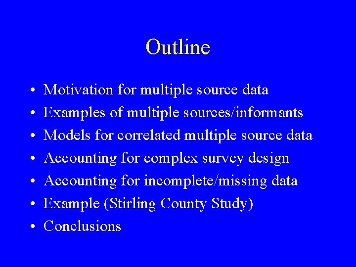
Outline • • Motivation for multiple source data Examples of multiple sources/informants Models for correlated multiple source data Accounting for complex survey design Accounting for incomplete/missing data Example (Stirling County Study) Conclusions

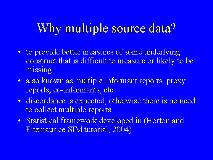
Why multiple source data? • to provide better measures of some underlying construct that is difficult to measure or likely to be missing • also known as multiple informant reports, proxy reports, co-informants, etc. • discordance is expected, otherwise there is no need to collect multiple reports • Statistical framework developed in (Horton and Fitzmaurice SIM tutorial, 2004)

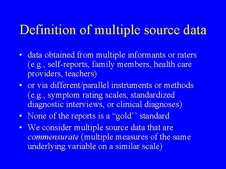
Definition of multiple source data • data obtained from multiple informants or raters (e. g. , self-reports, family members, health care providers, teachers) • or via different/parallel instruments or methods (e. g. , symptom rating scales, standardized diagnostic interviews, or clinical diagnoses) • None of the reports is a “gold’’ standard • We consider multiple source data that are commensurate (multiple measures of the same underlying variable on a similar scale)

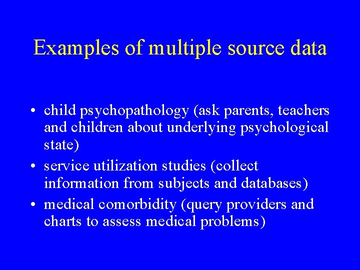
Examples of multiple source data • child psychopathology (ask parents, teachers and children about underlying psychological state) • service utilization studies (collect information from subjects and databases) • medical comorbidity (query providers and charts to assess medical problems)

Examples of multiple source data (cont. ) • adherence studies (collect self-report of adherence, electronic pill caps [MEMS] plus pharmacy records) • nutritional epidemiology (utilize multiple dietary instruments such as food frequency questionnaires, 24 -hour recalls, food diaries)

Incomplete/missing reports • Multiple source reports are commonly incomplete since, by definition, they are collected from sources other than the primary subject of the study • This missingness may be by design or happenstance (or both!)

Example: missing source reports • Consider service utilization studies that collect information from subjects and databases • Subjects may be lost to follow-up (or only contacted periodically) • Databases may be incomplete (lack of consent, lack of appropriate coverage)

Analytic approach • Multiple sources can provide information on outcomes or predictors (risk factors) • Multiple source outcome: what is the prevalence of child psychopathology? (measured using parallel parent and teacher reports) • Fitzmaurice et al (AJE, 1995), Horton et al (HSOR, 2002), Horton and Fitzmaurice (SIM tutorial, 2004)

Analytic approach (cont. ) • Multiple source predictor: what are the odds of developing depression in adulthood, conditional on parallel reports of anxiety (collected from a child and a parent)? • Examples: Horton et al (AJE, 2001), Lash et al (AJE, 2003), Liddicoat et al (JGIM, 2004), Horton and Fitzmaurice (SIM tutorial, 2004) • We will focus on an example using multiple source predictors

Notation • Let Y denote a univariate outcome for a given subject • Let denote the l’th multiple source predictor • Let Z denote a vector of other covariates for the subject • To simplify exposition, we consider two sources with dichotomous reports (L=2)

Questions to consider • Are the sources reporting on the same underlying construct (are they commensurate or interchangeable? ) • Is it possible to combine the reports in some fashion? • How to handle missing reports?

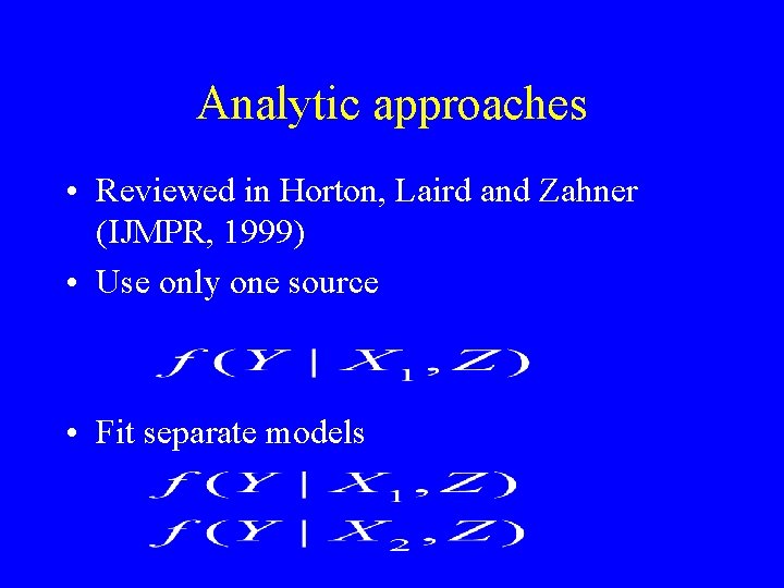
Analytic approaches • Reviewed in Horton, Laird and Zahner (IJMPR, 1999) • Use only one source • Fit separate models

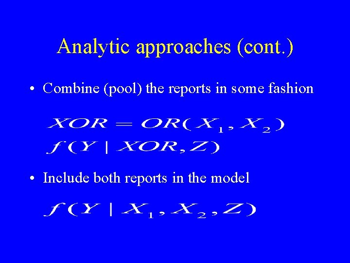
Analytic approaches (cont. ) • Combine (pool) the reports in some fashion • Include both reports in the model

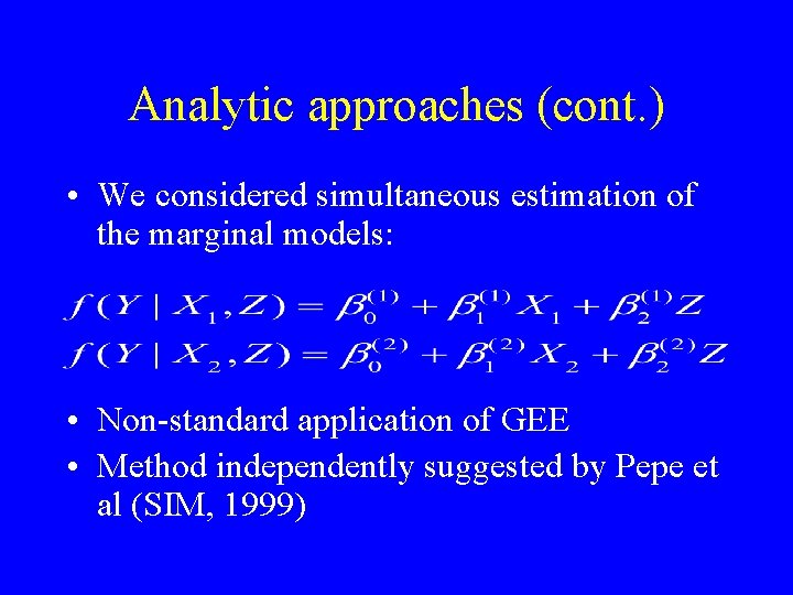
Analytic approaches (cont. ) • We considered simultaneous estimation of the marginal models: • Non-standard application of GEE • Method independently suggested by Pepe et al (SIM, 1999)

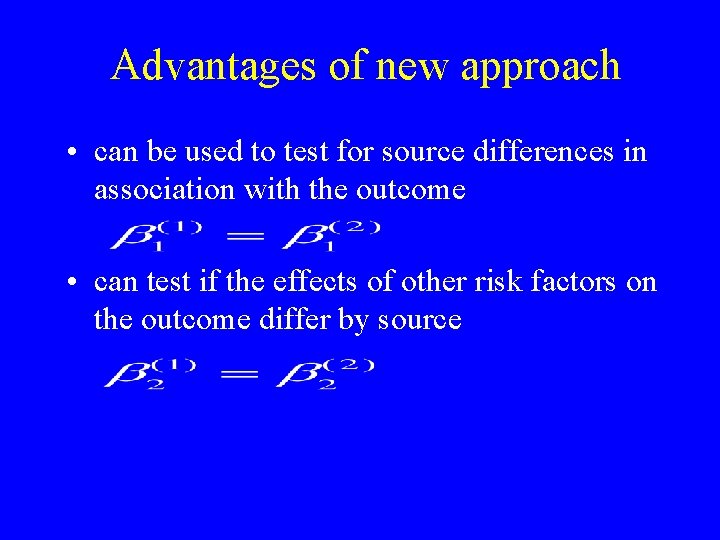
Advantages of new approach • can be used to test for source differences in association with the outcome • can test if the effects of other risk factors on the outcome differ by source

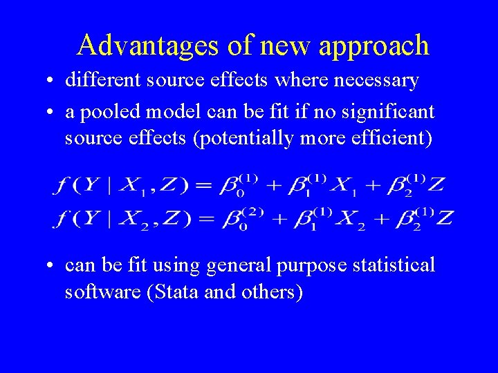
Advantages of new approach • different source effects where necessary • a pooled model can be fit if no significant source effects (potentially more efficient) • can be fit using general purpose statistical software (Stata and others)

Accounting for survey design • Many health services or epidemiologic studies arise from complex survey samples • Need to address stratification, multi-stage clustering and unequal sampling weights • Failing to properly account for survey design may lead to bias and incorrect estimation of variability

Accounting for survey design (cont. ) • Estimation proceeds using the approximate (quasi) log-likelihood (weighted version of the usual score equations for a GLM, accounting for the multi-stage clustering, including multiple source reports) • Can be fit using general purpose statistical software (elegant and powerful implementation in Stata)

Accounting for incomplete source reports • Missing source reports are missing predictors • Use weighted estimating equation methodology of Robins et al (JASA, 1994) and Xie and Paik (Biometrics, 1997), applied by Horton et al, (AJE, 2001) • Adds an additional “missingness weight” • Complications to variance estimation

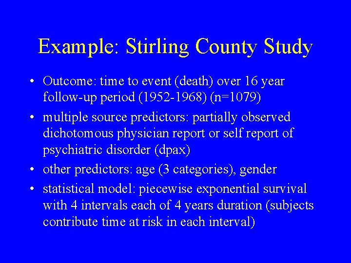
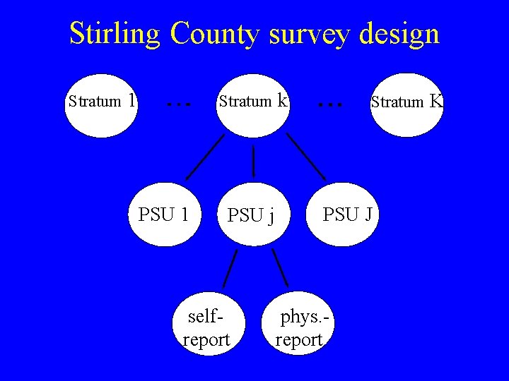
Example: Stirling County Study • Outcome: time to event (death) over 16 year follow-up period (1952 -1968) (n=1079) • multiple source predictors: partially observed dichotomous physician report or self report of psychiatric disorder (dpax) • other predictors: age (3 categories), gender • statistical model: piecewise exponential survival with 4 intervals each of 4 years duration (subjects contribute time at risk in each interval)

Stirling County survey design Strata Stratum 11 Stratum k PSU 1 PSU j selfreport Stratum K PSU J phys. report

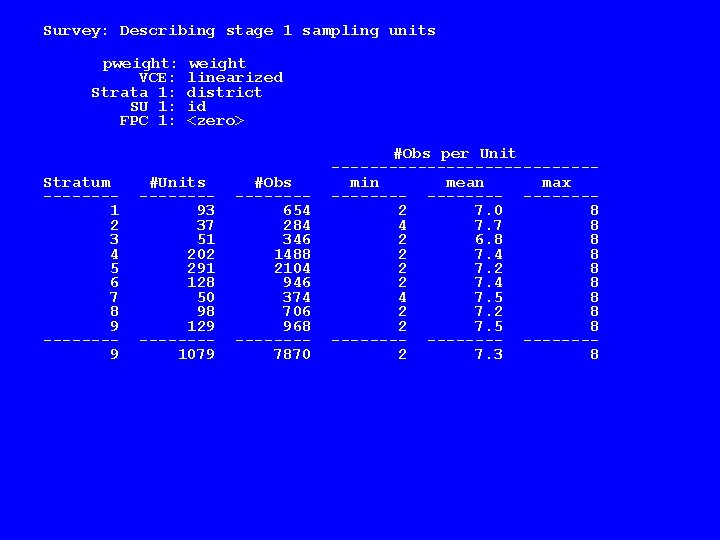
Implementation in Stata Specify probability sampling unit (subject), probability sampling weights (weight) and stratification variable (district): svyset id [pweight=weight], strata(district) Describe the sampling design: svydes

Survey: Describing stage 1 sampling units pweight: VCE: Strata 1: SU 1: FPC 1: Stratum -------1 2 3 4 5 6 7 8 9 -------9 weight linearized district id <zero> #Units -------93 37 51 202 291 128 50 98 129 -------1079 #Obs -------654 284 346 1488 2104 946 374 706 968 -------7870 #Obs per Unit --------------min mean max --------2 7. 0 8 4 7. 7 8 2 6. 8 8 2 7. 4 8 2 7. 2 8 2 7. 4 8 4 7. 5 8 2 7. 2 8 2 7. 5 8 --------2 7. 3 8

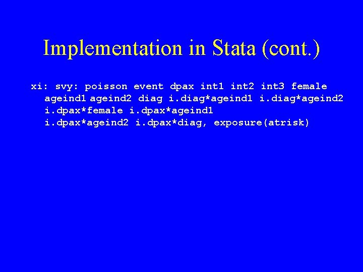
Implementation in Stata (cont. ) xi: svy: poisson event dpax int 1 int 2 int 3 female ageind 1 ageind 2 diag i. diag*ageind 1 i. diag*ageind 2 i. dpax*female i. dpax*ageind 1 i. dpax*ageind 2 i. dpax*diag, exposure(atrisk)

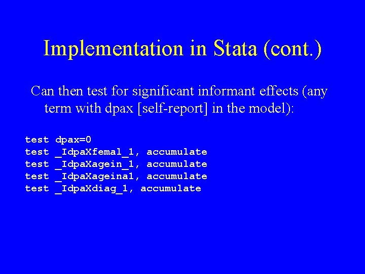
Implementation in Stata (cont. ) Can then test for significant informant effects (any term with dpax [self-report] in the model): test test dpax=0 _Idpa. Xfemal_1, accumulate _Idpa. Xageina 1, accumulate _Idpa. Xdiag_1, accumulate

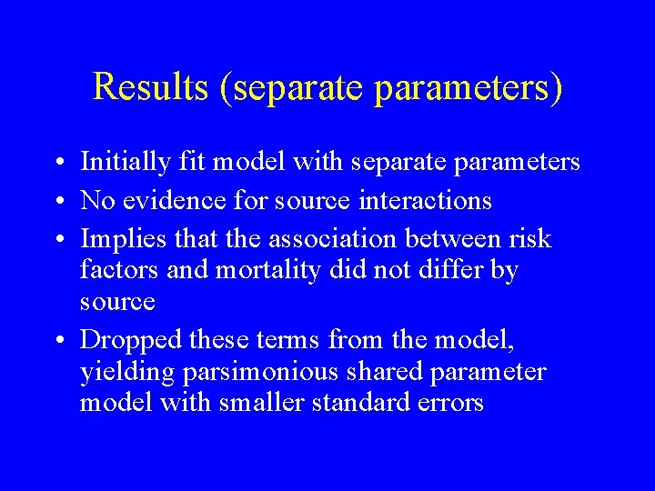
Results (separate parameters) • Initially fit model with separate parameters • No evidence for source interactions • Implies that the association between risk factors and mortality did not differ by source • Dropped these terms from the model, yielding parsimonious shared parameter model with smaller standard errors

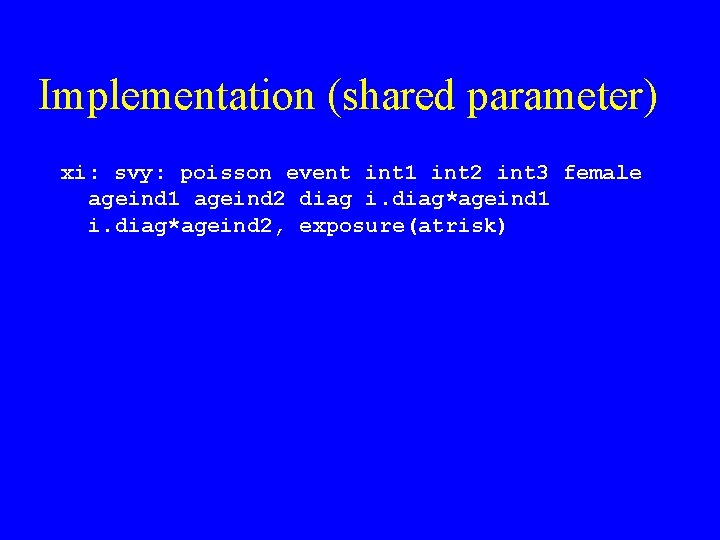
Implementation (shared parameter) xi: svy: poisson event int 1 int 2 int 3 female ageind 1 ageind 2 diag i. diag*ageind 1 i. diag*ageind 2, exposure(atrisk)

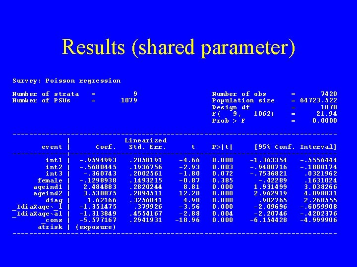
Results (shared parameter) Survey: Poisson regression Number of strata Number of PSUs = = 9 1079 Number of obs Population size Design df F( 9, 1062) Prob > F = 7420 = 64723. 522 = 1070 = 21. 94 = 0. 0000 ---------------------------------------| Linearized event | Coef. Std. Err. t P>|t| [95% Conf. Interval] -------+--------------------------------int 1 | -. 9594993. 2058191 -4. 66 0. 000 -1. 363354 -. 5556444 int 2 | -. 5680445. 1936756 -2. 93 0. 003 -. 9480716 -. 1880174 int 3 | -. 360743. 2002561 -1. 80 0. 072 -. 7536821. 0321962 female | -. 1298938. 1493215 -0. 87 0. 385 -. 42289. 1631024 ageind 1 | 2. 484883. 2820244 8. 81 0. 000 1. 931499 3. 038266 ageind 2 | 3. 530875. 2894511 12. 20 0. 000 2. 962919 4. 098831 diag | 1. 62166. 3256041 4. 98 0. 000. 982765 2. 260555 _Idia. Xage~_1 | -1. 351475. 379926 -3. 56 0. 000 -2. 09696 -. 6059908 _Idia. Xage~a 1 | -1. 313849. 4554167 -2. 88 0. 004 -2. 20746 -. 4202376 _cons | -5. 577167. 2941931 -18. 96 0. 000 -6. 154428 -4. 999906 atrisk | (exposure) ---------------------------------------

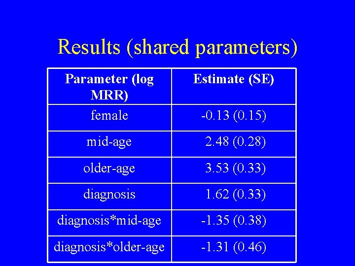
Results (shared parameters) Parameter (log MRR) female Estimate (SE) mid-age 2. 48 (0. 28) older-age 3. 53 (0. 33) diagnosis 1. 62 (0. 33) diagnosis*mid-age -1. 35 (0. 38) diagnosis*older-age -1. 31 (0. 46) -0. 13 (0. 15)

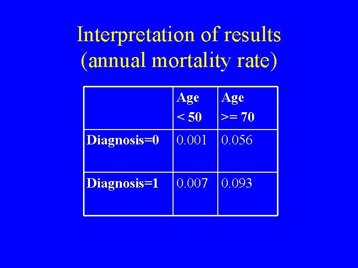
Interpretation of results (annual mortality rate) Age < 50 Age >= 70 Diagnosis=0 0. 001 0. 056 Diagnosis=1 0. 007 0. 093

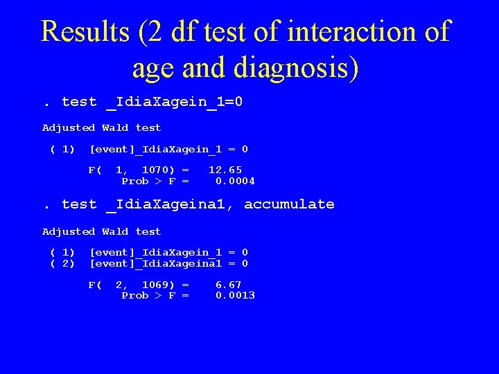
Results (2 df test of interaction of age and diagnosis). test _Idia. Xagein_1=0 Adjusted Wald test ( 1) [event]_Idia. Xagein_1 = 0 F( 1, 1070) = Prob > F = 12. 65 0. 0004 . test _Idia. Xageina 1, accumulate Adjusted Wald test ( 1) ( 2) [event]_Idia. Xagein_1 = 0 [event]_Idia. Xageina 1 = 0 F( 2, 1069) = Prob > F = 6. 67 0. 0013

Results (calculation of MRR and 95% CI). lincom diag, eform ( 1) [event]diag = ---------------------------------event | exp(b) Std. Err. t P>|t| [95% Conf. Interval] ------+-----------------------------(1) | 5. 0615 1. 6480 4. 98 0. 000 2. 6718 9. 5884 --------------------------------- . lincom diag + _Idia. Xagein_1, eform ( 1) [event]diag + [event]_Idia. Xagein_1 = 0 ---------------------------------event | exp(b) Std. Err. t P>|t| [95% Conf. Interval] ------+-----------------------------(1) | 1. 3102. 25297 1. 40 0. 162. 89703 1. 9137 ---------------------------------

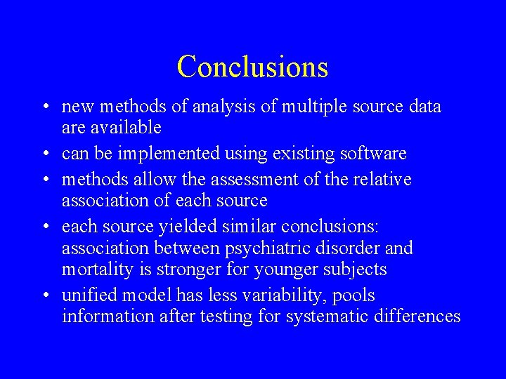
Conclusions • new methods of analysis of multiple source data are available • can be implemented using existing software • methods allow the assessment of the relative association of each source • each source yielded similar conclusions: association between psychiatric disorder and mortality is stronger for younger subjects • unified model has less variability, pools information after testing for systematic differences

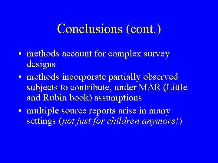
Conclusions (cont. ) • methods account for complex survey designs • methods incorporate partially observed subjects to contribute, under MAR (Little and Rubin book) assumptions • multiple source reports arise in many settings (not just for children anymore!)

Future work • Maximum-likelihood estimation instead of GEE approach – May yield efficiency gains – Particularly useful for missing reports • Non-commensurate reports – Different scales – Different underlying constructs – Consider latent variable models (e. g. work of Normand colleagues) – See also gllamm and forthcoming Stata book by Rabe-Hesketh and Skrondal)

Analysis of multiple informant/ multiple source data in Stata Nicholas Horton Department of Mathematics Smith College, Northampton MA nhorton at email. smith. edu http: //www. biostat. harvard. edu/multinform