Analysis of microarray data with BASE Julien Gagneur

Analysis of microarray data with BASE Julien Gagneur 17 th March 2006

Motivation - Central depository of micro-array data: http: //embase. embl. de/base/ - Standard data analysis feasible - Traceability of data manipulation

Data loading - Data must be correctly loaded into BASE - This implies annotations of : - The array (plate, reporter, design) - The biomaterials (samples, extract) - Hybridization (which biomaterial on which array) - Charles provides guidelines for that - Tedious yet important for: - publication - downstream analysis

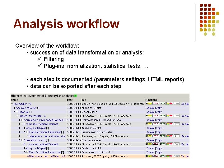
Analysis workflow Overview of the workflow: • succession of data transformation or analysis: ü Filtering ü Plug-ins: normalization, statistical tests, … • each step is documented (parameters settings, HTML reports) • data can be exported after each step

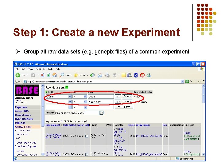
Step 1: Create a new Experiment Ø Group all raw data sets (e. g. genepix files) of a common experiment

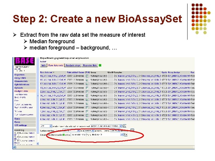
Step 2: Create a new Bio. Assay. Set Ø Extract from the raw data set the measure of interest Ø Median foreground Ø median foreground – background, …

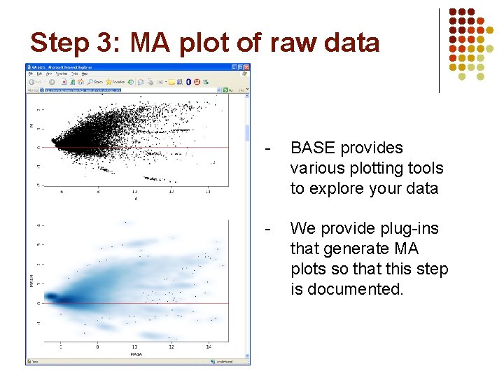
Step 3: MA plot of raw data - BASE provides various plotting tools to explore your data - We provide plug-ins that generate MA plots so that this step is documented.

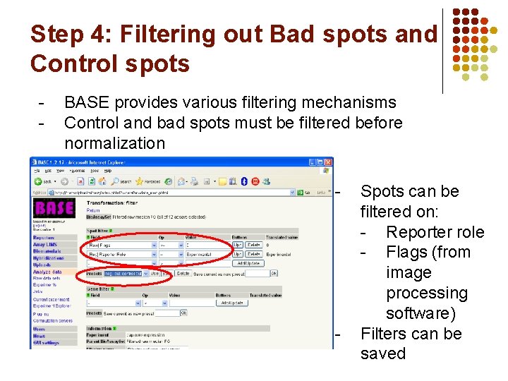
Step 4: Filtering out Bad spots and Control spots - BASE provides various filtering mechanisms Control and bad spots must be filtered before normalization - - Spots can be filtered on: - Reporter role - Flags (from image processing software) Filters can be saved

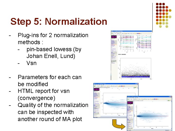
Step 5: Normalization - Plug-ins for 2 normalization methods : - pin-based lowess (by Johan Enell, Lund) - Vsn - Parameters for each can be modified HTML report for vsn (convergence) Quality of the normalization can be inspected with another round of MA plot -

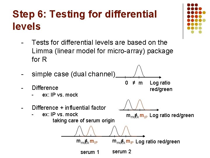
Step 6: Testing for differential levels - Tests for differential levels are based on the Limma (linear model for micro-array) package for R - simple case (dual channel) - Difference - - 0 ≠ m ex: IP vs. mock Log ratio red/green Difference + influential factor - ex: IP vs. mock taking care of serum origin mmock ≠ m. IP serum 1 mmock ≠ m. IP Log ratio red/green serum 2

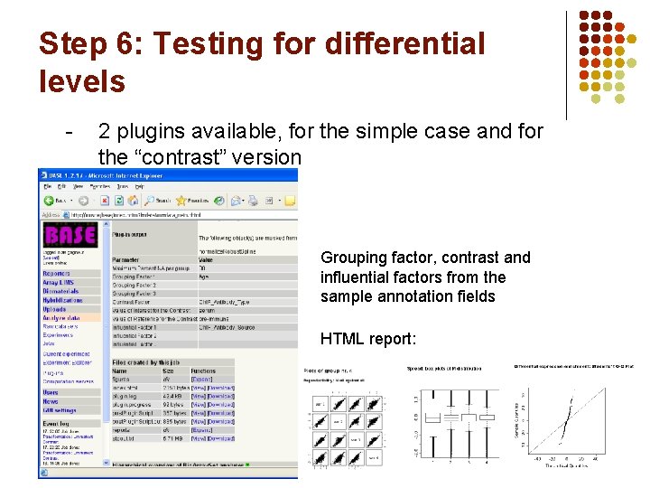
Step 6: Testing for differential levels - 2 plugins available, for the simple case and for the “contrast” version Grouping factor, contrast and influential factors from the sample annotation fields HTML report:

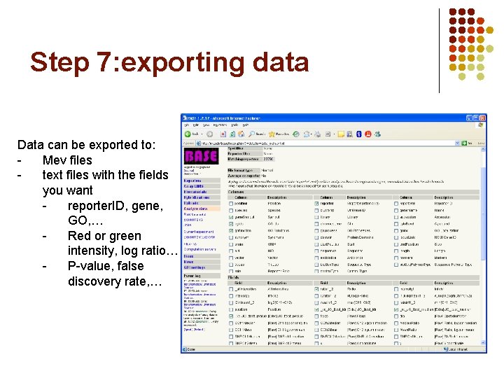
Step 7: exporting data Data can be exported to: Mev files text files with the fields you want reporter. ID, gene, GO, … Red or green intensity, log ratio… P-value, false discovery rate, …

Conclusion Complete overview/control on steps : • all parameters used in applications or filters are stored • data can be browsed at each step and plotted • you can share or not your analysis results • provide a powerful way to centralize QA results • data can be exported at any time Standard tools are available Further plug-ins based on R packages can be developed easily.