Analysis of Large Graphs Community Detection By KIM

Analysis of Large Graphs Community Detection By: KIM HYEONGCHEOL WALEED ABDULWAHAB YAHYA AL-GOBI MUHAMMAD BURHAN HAFEZ SHANG XINDI HE RUIDAN 1

Overview 2 Introduction & Motivation Graph cut criterion Min-cut Normalized-cut Non-overlapping community detection Spectral clustering Deep auto-encoder Overlapping community detection Big. CLAM algorithm

1 Introduction Objective Intro to Analysis of Large Graphs KIM HYEONG CHEOL

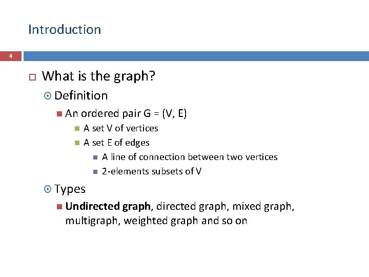
Introduction 4 What is the graph? Definition An ordered pair G = (V, E) A set V of vertices A set E of edges A line of connection between two vertices 2 -elements subsets of V Types Undirected graph, mixed graph, multigraph, weighted graph and so on

Introduction 5 Undirected graph Edges have no orientation Edge (x, y) = Edge (y, x) The maximum number of edges : n(n-1)/2 All pair of vertices are connected to each other Undirected graph G = (V, E) V : {1, 2, 3, 4, 5, 6} E : {E(1, 2), E(2, 3), E(1, 5), E(2, 5), E(4, 5) E(3, 4), E(4, 6)}

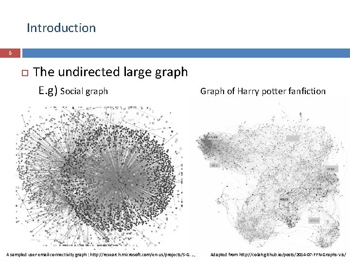
Introduction 6 The undirected large graph E. g) Social graph Graph of Harry potter fanfiction A sampled user email-connectivity graph : http: //research. microsoft. com/en-us/projects/S-GPS/ Adapted from http: //colah. github. io/posts/2014 -07 -FFN-Graphs-Vis/

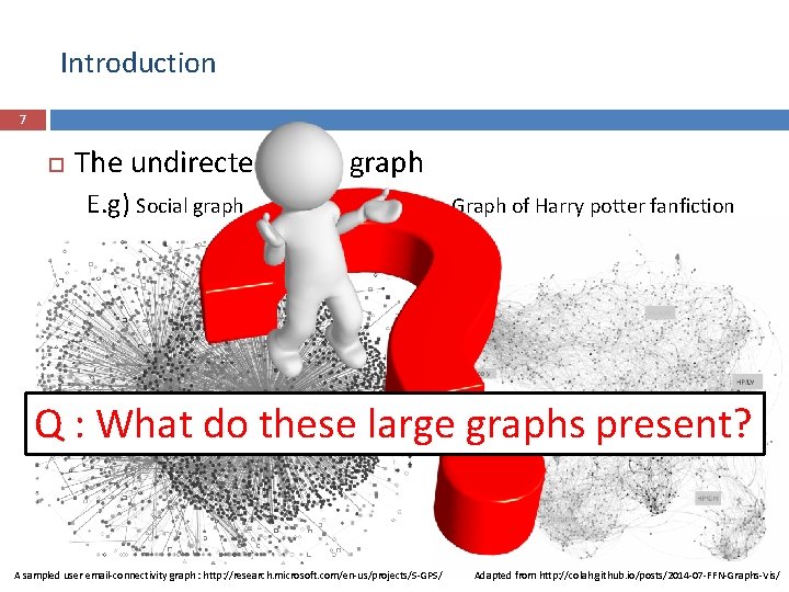
Introduction 7 The undirected large graph E. g) Social graph Graph of Harry potter fanfiction Q : What do these large graphs present? A sampled user email-connectivity graph : http: //research. microsoft. com/en-us/projects/S-GPS/ Adapted from http: //colah. github. io/posts/2014 -07 -FFN-Graphs-Vis/

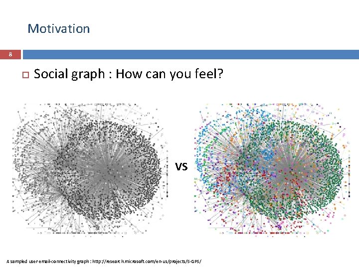
Motivation 8 Social graph : How can you feel? VS A sampled user email-connectivity graph : http: //research. microsoft. com/en-us/projects/S-GPS/

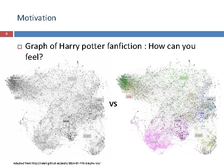
Motivation 9 Graph of Harry potter fanfiction : How can you feel? VS Adapted from http: //colah. github. io/posts/2014 -07 -FFN-Graphs-Vis/

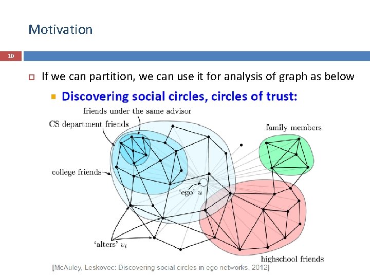
Motivation 10 If we can partition, we can use it for analysis of graph as below

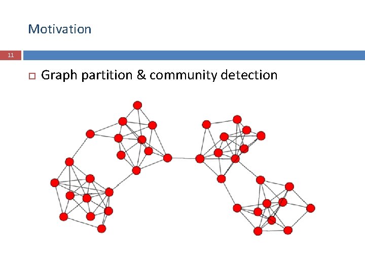
Motivation 11 Graph partition & community detection

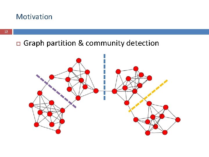
Motivation 12 Graph partition & community detection

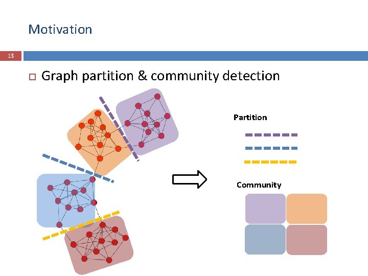
Motivation 13 Graph partition & community detection Partition Community

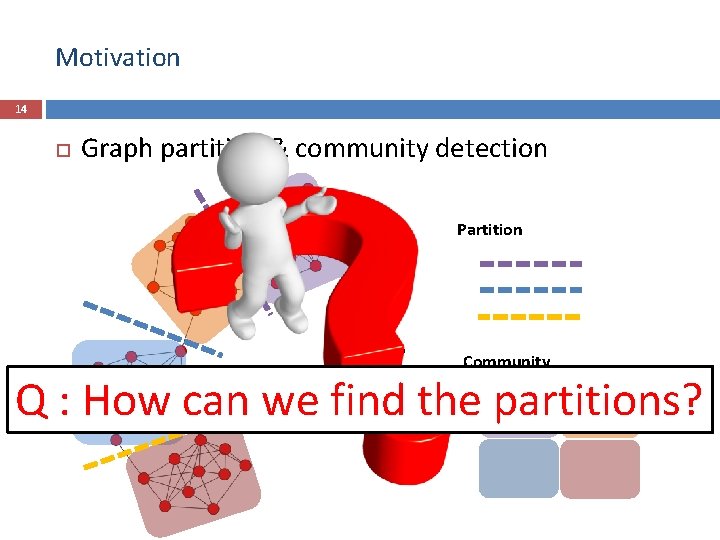
Motivation 14 Graph partition & community detection Partition Community Q : How can we find the partitions?

2 Minimum-cut Normalized-cut Criterion : Graph partitioning KIM HYEONG CHEOL

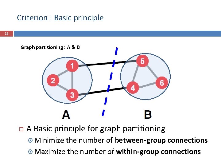
Criterion : Basic principle 16 Graph partitioning : A & B A Basic principle for graph partitioning Minimize the number of between-group connections Maximize the number of within-group connections

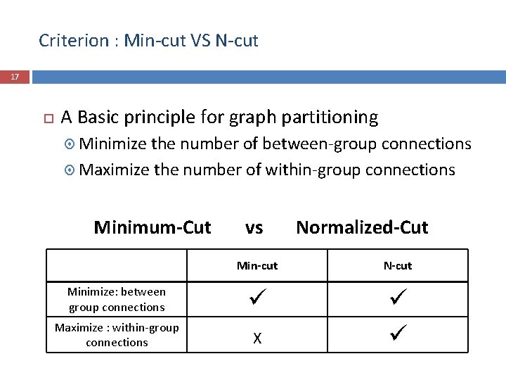
Criterion : Min-cut VS N-cut 17 A Basic principle for graph partitioning Minimize the number of between-group connections Maximize the number of within-group connections Minimum-Cut Minimize: between group connections Maximize : within-group connections vs Normalized-Cut Min-cut N-cut ü X ü ü

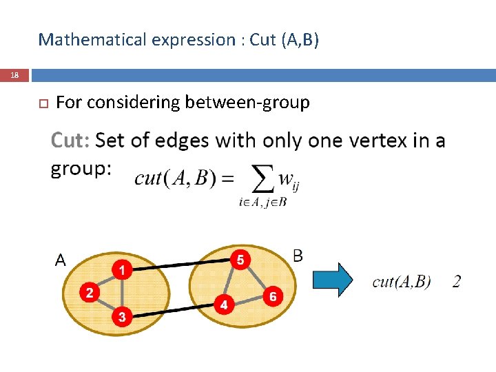
Mathematical expression : Cut (A, B) 18 For considering between-group

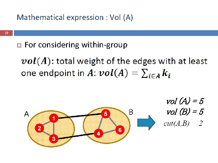
Mathematical expression : Vol (A) 19 For considering within-group vol (A) = 5 vol (B) = 5

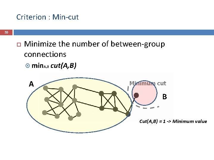
Criterion : Min-cut 20 Minimize the number of between-group connections min. A, B cut(A, B) A B Cut(A, B) = 1 -> Minimum value

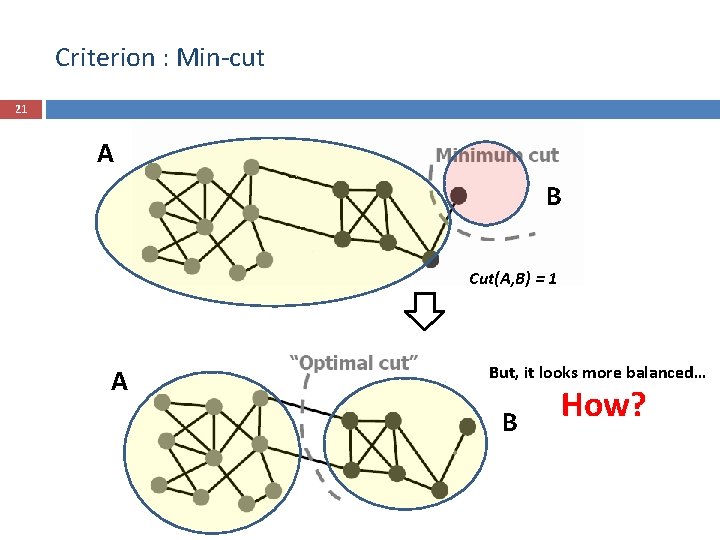
Criterion : Min-cut 21 A B Cut(A, B) = 1 A But, it looks more balanced… B How?

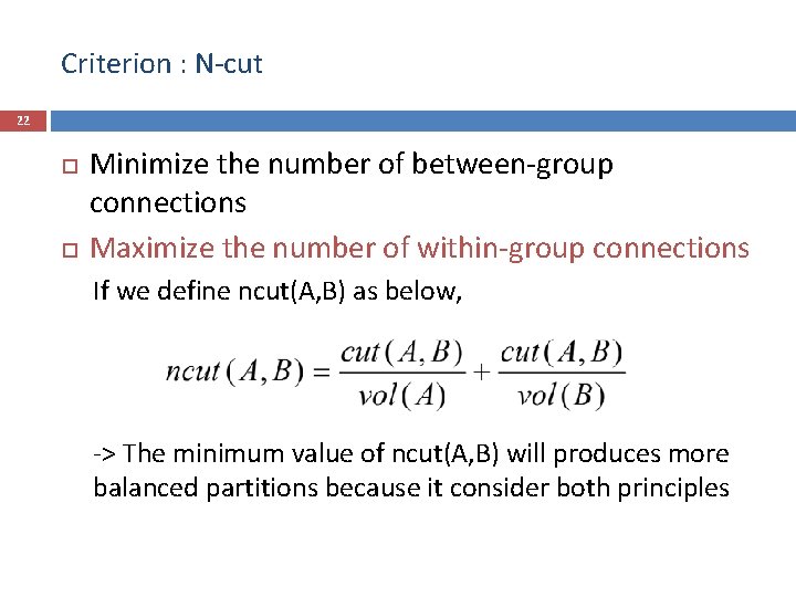
Criterion : N-cut 22 Minimize the number of between-group connections Maximize the number of within-group connections If we define ncut(A, B) as below, -> The minimum value of ncut(A, B) will produces more balanced partitions because it consider both principles

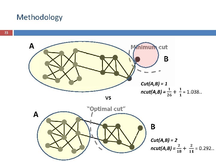
Methodology 23 A B VS A B

Summary 24 What is the undirected large graph? How can we get insight from the undirected large graph? Graph Partition & Community detection What were the methodology for good graph partition? Min-cut Normalized-cut

3 Spectral Clustering Deep Graph. Encoder Non-overlapping community detection: Waleed Abdulwahab Yahya Al-Gobi

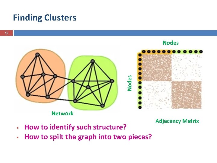
Finding Clusters 26 Nodes Network § § How to identify such structure? How to spilt the graph into two pieces? Adjacency Matrix

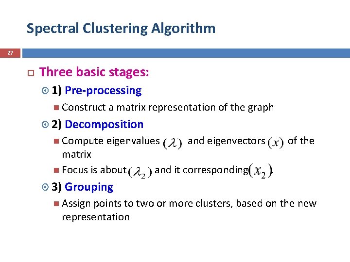
Spectral Clustering Algorithm 27 Three basic stages: 1) Pre-processing Construct a matrix representation of the graph 2) Decomposition Compute eigenvalues and eigenvectors of the matrix Focus is about and it corresponding . 3) Grouping Assign points to two or more clusters, based on the new representation

Matrix Representations 28 Adjacency matrix (A): n n binary matrix A=[aij], aij=1 if edge between node i and j 5 1 2 3 4 6 1 2 3 4 5 6 1 0 1 0 2 1 0 0 0 3 1 1 0 0 4 0 0 1 1 5 1 0 0 1 6 0 0 0 1 1 0

Matrix Representations 29 Degree matrix (D): n n diagonal matrix D=[dii], dii = degree of node i 5 1 2 3 4 6 1 2 3 4 5 6 1 3 0 0 0 2 0 0 3 0 0 0 4 0 0 0 3 0 0 5 0 0 3 0 6 0 0 0 2

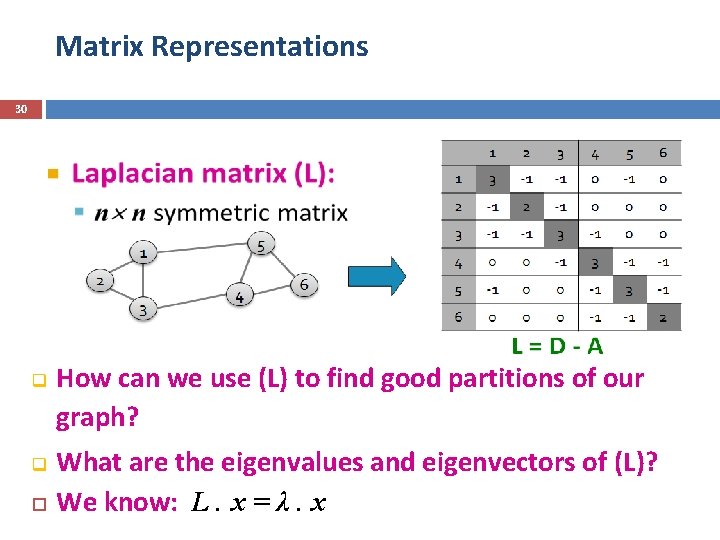
Matrix Representations 30 q q How can we use (L) to find good partitions of our graph? What are the eigenvalues and eigenvectors of (L)? We know: L. x = λ. x

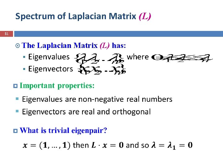
Spectrum of Laplacian Matrix (L) 31 The Laplacian Matrix (L) has: Eigenvalues where § Eigenvectors §

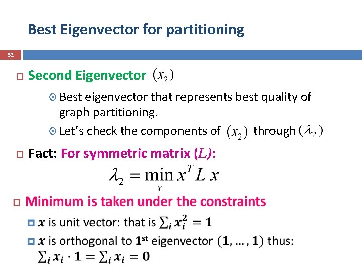
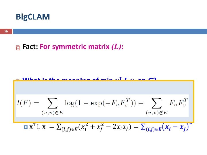
Best Eigenvector for partitioning 32 Second Eigenvector Best eigenvector that represents best quality of graph partitioning. Let’s check the components of through Fact: For symmetric matrix (L):

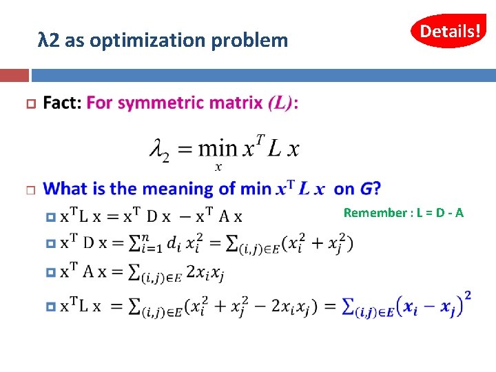
λ 2 as optimization problem Details! Remember : L = D - A 33

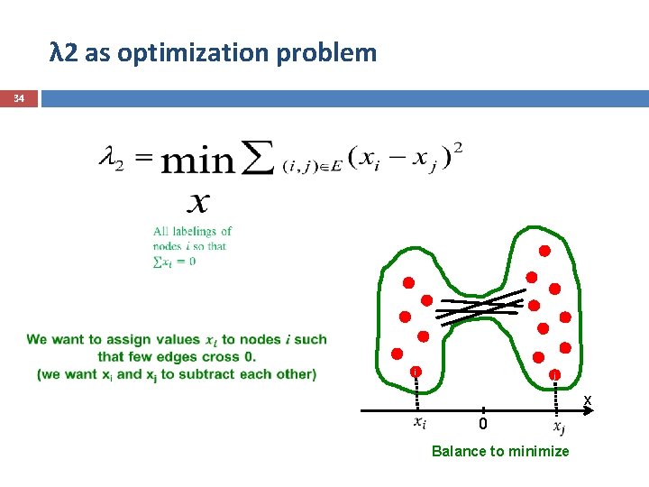
λ 2 as optimization problem 34 i j x 0 Balance to minimize

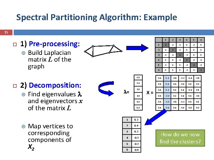
Spectral Partitioning Algorithm: Example 35 2 3 4 5 6 1 3 -1 -1 0 2 -1 0 0 0 3 -1 -1 3 -1 0 0 4 0 0 -1 3 -1 -1 5 -1 0 0 -1 3 -1 6 0 0 0 -1 -1 2 0. 0 0. 4 0. 3 -0. 5 -0. 2 -0. 4 -0. 5 1. 0 0. 4 0. 6 0. 4 -0. 4 0. 0 0. 4 0. 3 0. 1 0. 6 -0. 4 0. 5 0. 4 -0. 3 0. 1 0. 6 0. 4 -0. 5 4. 0 0. 4 -0. 3 -0. 5 -0. 2 0. 4 0. 5 5. 0 0. 4 -0. 6 0. 4 -0. 4 0. 0 1) Pre-processing: 1 Build Laplacian matrix L of the graph 2) Decomposition: Find eigenvalues and eigenvectors x of the matrix L Map vertices to corresponding components of X 2 = 3. 0 1 0. 3 2 0. 6 3 0. 3 4 -0. 3 5 -0. 3 6 -0. 6 X= How do we now find the clusters?

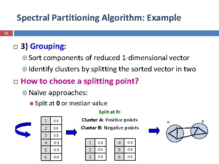
Spectral Partitioning Algorithm: Example 36 3) Grouping: Sort components of reduced 1 -dimensional vector Identify clusters by splitting the sorted vector in two How to choose a splitting point? Naïve approaches: Split at 0 or median value Split at 0: Cluster A: Positive points Cluster B: Negative points 1 0. 3 2 0. 6 3 0. 3 4 -0. 3 1 0. 3 4 -0. 3 5 -0. 3 2 0. 6 5 -0. 3 6 -0. 6 3 0. 3 6 -0. 6 A B

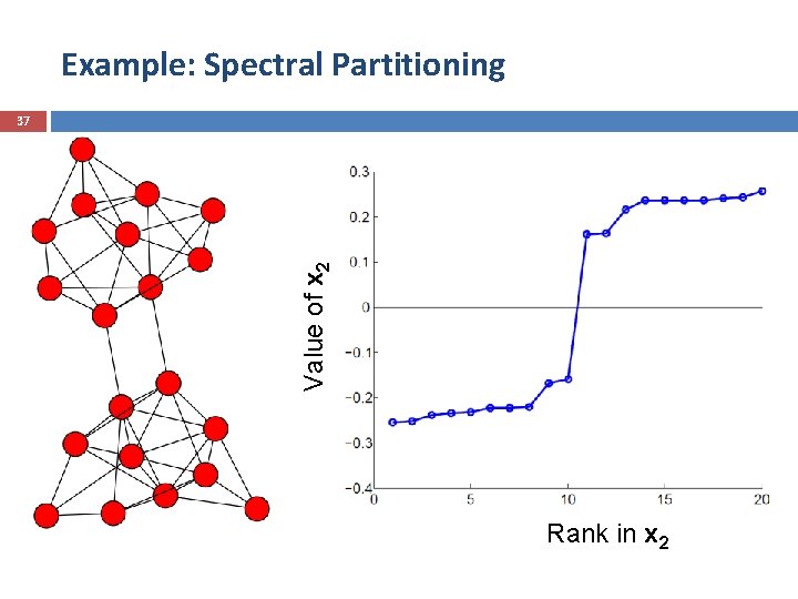
Example: Spectral Partitioning Value of x 2 37 Rank in x 2

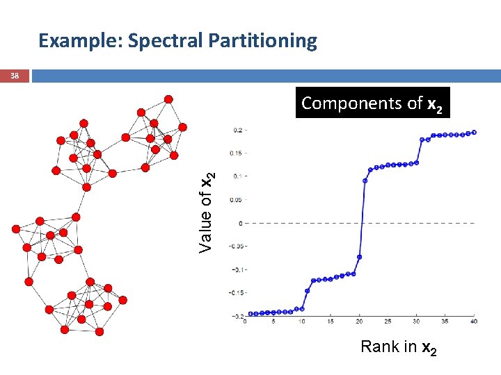
Example: Spectral Partitioning 38 Value of x 2 Components of x 2 Rank in x 2

k-Way Spectral Clustering 39 How do we partition a graph into k clusters? Two basic approaches: Recursive bi-partitioning [Hagen et al. , ’ 92] Recursively apply bi-partitioning algorithm in a hierarchical divisive manner Disadvantages: Inefficient Cluster multiple eigenvectors [Shi-Malik, ’ 00] Build a reduced space from multiple eigenvectors Commonly used in recent papers A preferable approach

4 Spectral Clustering Deep Graph. Encoder [Tian et al. , 2014] Muhammad Burhan Hafez

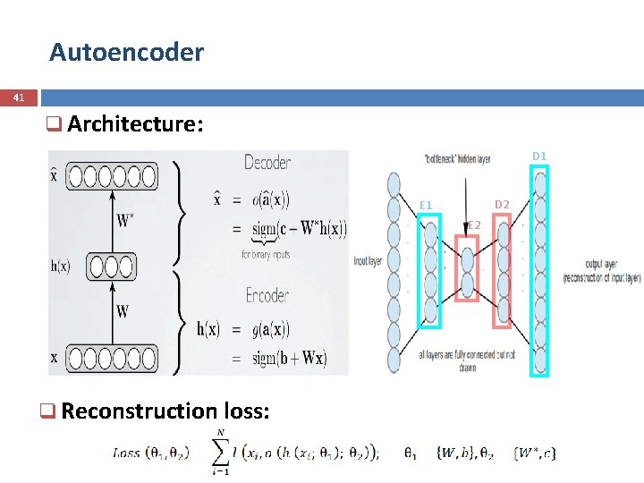
Autoencoder 41 q Architecture: D 1 D 2 E 1 E 2 q Reconstruction loss:

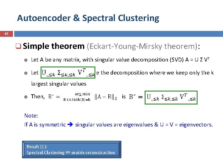
Autoencoder & Spectral Clustering 42 q Simple theorem (Eckart-Young-Mirsky theorem): Let A be any matrix, with singular value decomposition (SVD) A = U Σ VT Let be the decomposition where we keep only the k largest singular values Then, is Note: If A is symmetric singular values are eigenvalues & U = V = eigenvectors. Result (1): Spectral Clustering ⇔ matrix reconstruction

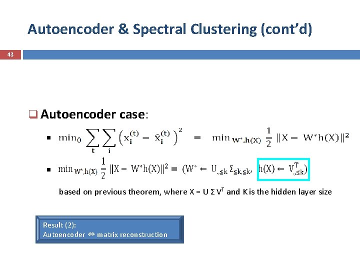
Autoencoder & Spectral Clustering (cont’d) 43 q Autoencoder case: § § based on previous theorem, where X = U Σ VT and K is the hidden layer size Result (2): Autoencoder ⇔ matrix reconstruction

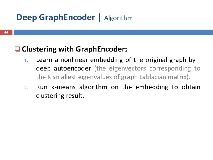
Deep Graph. Encoder | Algorithm 44 q Clustering with Graph. Encoder: 1. 2. Learn a nonlinear embedding of the original graph by deep autoencoder (the eigenvectors corresponding to the K smallest eigenvalues of graph Lablacian matrix). Run k-means algorithm on the embedding to obtain clustering result.

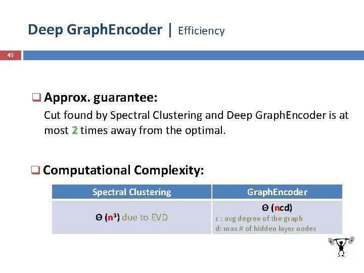
Deep Graph. Encoder | Efficiency 45 q Approx. guarantee: Cut found by Spectral Clustering and Deep Graph. Encoder is at most 2 times away from the optimal. q Computational Complexity: Spectral Clustering Θ (n 3) due to EVD Graph. Encoder Θ (ncd) c : avg degree of the graph d: max # of hidden layer nodes

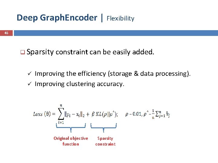
Deep Graph. Encoder | Flexibility 46 q Sparsity constraint can be easily added. ü Improving the efficiency (storage & data processing). ü Improving clustering accuracy. Original objective function Sparsity constraint

5 Big. CLAM: Introduction Overlapping Community Detection SHANG XINDI

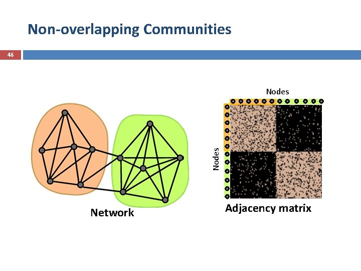
Non-overlapping Communities 48 Nodes Network Adjacency matrix

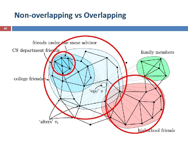
Non-overlapping vs Overlapping 49

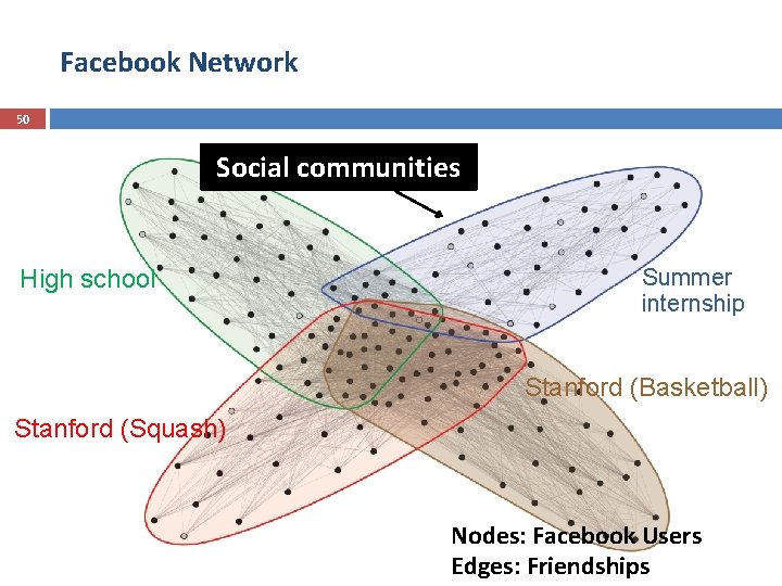
Facebook Network 50 Social communities High school Summer internship Stanford (Basketball) Stanford (Squash) Nodes: Facebook Users Edges: Friendships 50

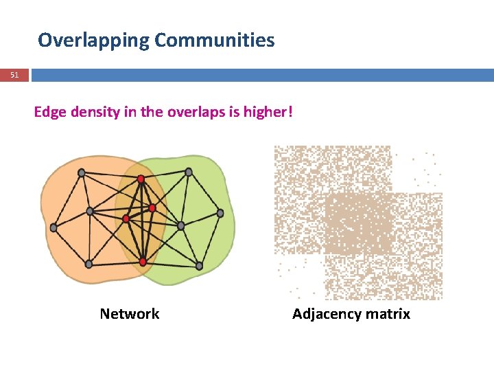
Overlapping Communities 51 Edge density in the overlaps is higher! Network Adjacency matrix

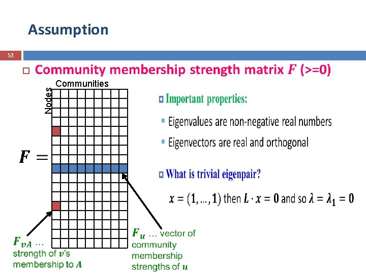
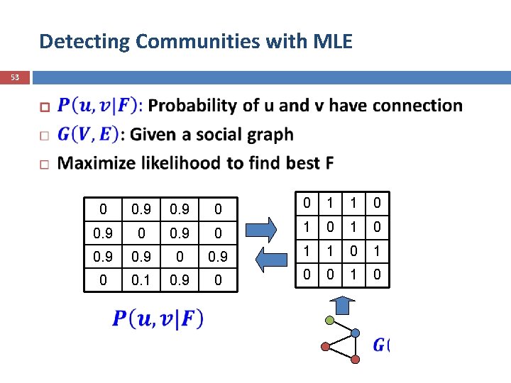
Assumption 52 Nodes Communities j

Detecting Communities with MLE 53 0 0. 9 0 0 1 1 0 0. 9 0 0. 9 1 1 0 0. 1 0. 9 0 0 0 1 0

Detecting Communities with MLE 54

Big. CLAM 55 Yang, Jaewon, and Jure Leskovec. "Overlapping community detection at scale: a nonnegative matrix factorization approach. " Proceedings of the sixth ACM international conference on Web search and data mining. ACM, 2013.

Big. CLAM 56

5 Big. CLAM: How to optimize parameter F ? Additional reading: state of the art methods Overlapping Community Detection He Ruidan

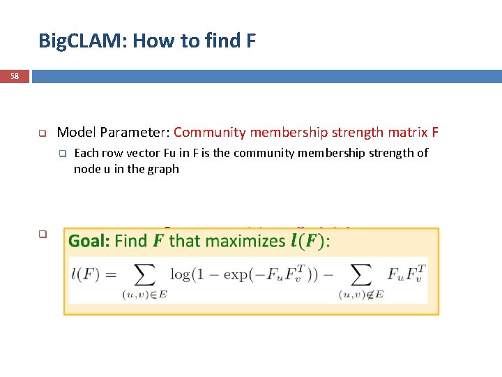
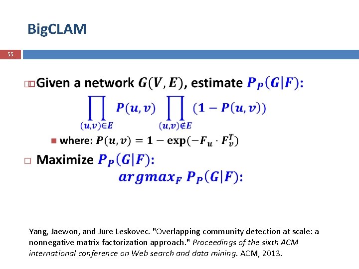
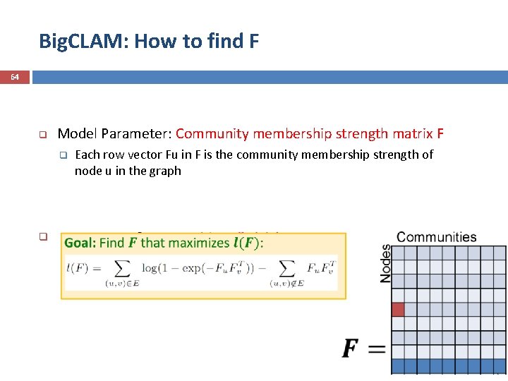
Big. CLAM: How to find F 58 q Model Parameter: Community membership strength matrix F q q Each row vector Fu in F is the community membership strength of node u in the graph

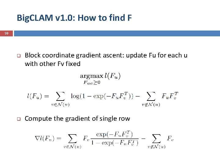
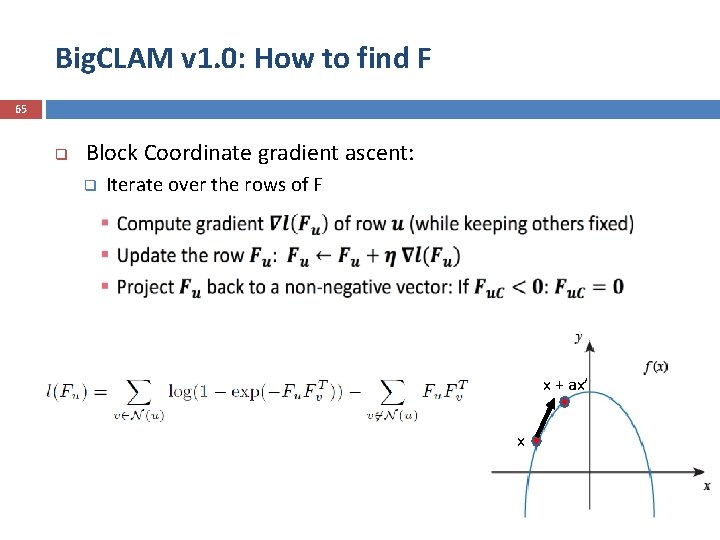
Big. CLAM v 1. 0: How to find F 59 q q Block coordinate gradient ascent: update Fu for each u with other Fv fixed Compute the gradient of single row

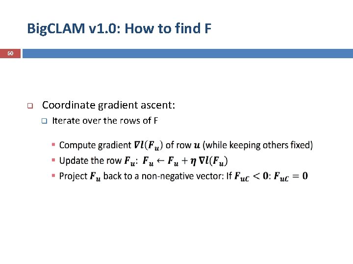
Big. CLAM v 1. 0: How to find F 60 q Coordinate gradient ascent: q Iterate over the rows of F

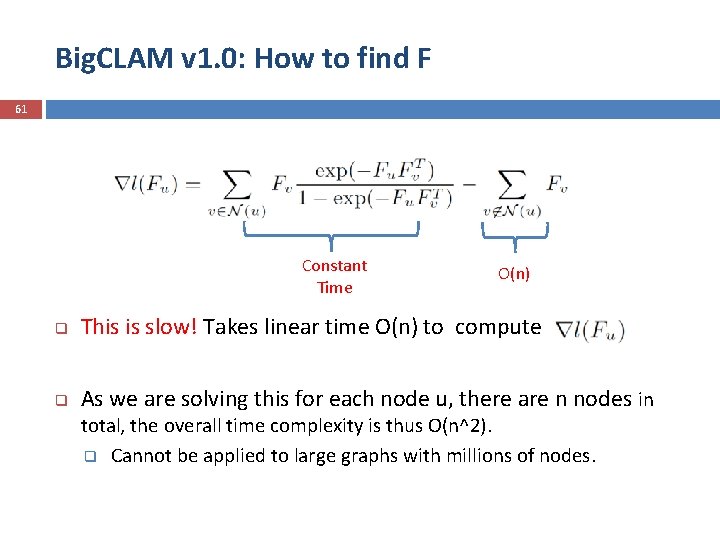
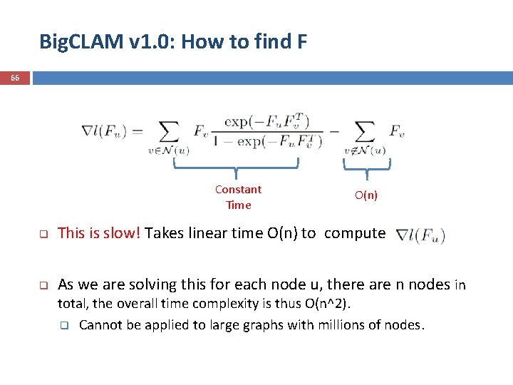
Big. CLAM v 1. 0: How to find F 61 Constant Time O(n) q This is slow! Takes linear time O(n) to compute q As we are solving this for each node u, there are n nodes in total, the overall time complexity is thus O(n^2). q Cannot be applied to large graphs with millions of nodes.

Big. CLAM v 2. 0: How to find F 62 q q q However, we notice that: Usually, the average degree of node in a graph could be treat as constant, Then it takes constant time to compute Therefore, time complexity to update matrix F is reduced to O(n)

6 Big. CLAM: How to optimize parameter F ? Additional reading: state of the art methods Overlapping Community Detection He Ruidan

Big. CLAM: How to find F 64 q Model Parameter: Community membership strength matrix F q q Each row vector Fu in F is the community membership strength of node u in the graph

Big. CLAM v 1. 0: How to find F 65 q Block Coordinate gradient ascent: q Iterate over the rows of F x + ax’ x

Big. CLAM v 1. 0: How to find F 66 Constant Time O(n) q This is slow! Takes linear time O(n) to compute q As we are solving this for each node u, there are n nodes in total, the overall time complexity is thus O(n^2). q Cannot be applied to large graphs with millions of nodes.

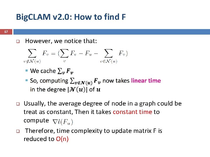
Big. CLAM v 2. 0: How to find F 67 q q q However, we notice that: Usually, the average degree of node in a graph could be treat as constant, Then it takes constant time to compute Therefore, time complexity to update matrix F is reduced to O(n)

5 Big. CLAM: How to optimize parameter F ? Additional reading: state of the art methods Overlapping Community Detection He Ruidan

Graph Representation 69 q Representation learning of graph node. q Try to represent each node using as a numerical vector. Given a graph, the vectors should be learned automatically. q Learning objective: The representation vectors for nodes share similar connections are close to each other in the vector space q After the representation of each node is learnt. Community detection could be modeled as a clustering / classification problem.

Graph Representation 70 q Graph representation using neural networks / deep learning q B. Perozzi, R. Al-Rfou, and S. Skiena. Deepwalk: Online learning of social representations. In SIGKDD, pages 701– 710. ACM, 2014. q J. Tang, M. Qu, M. Wang, M. Zhang, J. Yan, and Q. Mei. Line: Large-scale information network embedding. In WWW. ACM, 2015. q F. Tian, B. Gao, Q. Cui, E. Chen, and T. -Y. Liu. Learning deep representations for graph clustering. In AAAI, 2014.

Summary 71 Introduction & Motivation Graph cut criterion Min-cut Normalized-cut Non-overlapping community detection Spectral clustering Deep auto-encoder Overlapping community detection Big. CLAM algorithm

72 Appendix

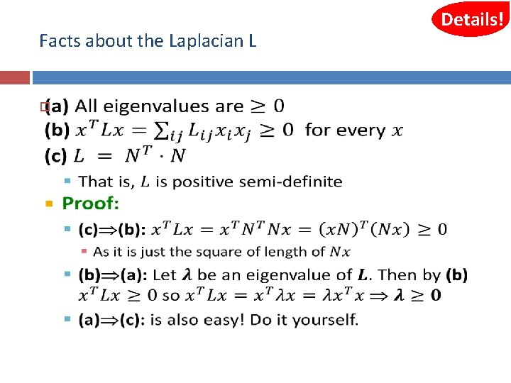
Facts about the Laplacian L Details! 73

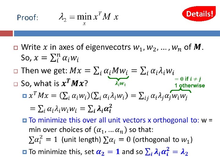
Details! Proof: 74