Analysis of HighDimensional Proteomics Data Networks and Topological

Analysis of High-Dimensional Proteomics Data: Networks and Topological Data Analysis Austin Chan, Janet Loyola, Iyesha Puri, Sophia Su, Roger Zhou

Stickleback fish

Scientific Question / Reasoning ● What is the goal of this project? ○ ● Association between protein expression of stickleback fish and environment What do we hope to find? ○ Do proteins appear jointly? Are there specific patterns of protein abundances among different environments? ○ Discover some underlying features or structures that are consistent throughout the analysis

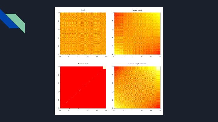
What do the data look like? ● ● ● High-Dimensional Objects ○ 1505 different proteins ○ 96 fish from 4 different environments ○ Hence, 24 fish for 1 environment Low sample size ○ Number of variables is significantly larger than the sample size ○ Large P, small n ○ Low sample size is problematic due to larger variance in the data Correlation - Distance matrix ○ Used to compare the relationships between each protein

What do the data look like? (cont. ) Protein 1 Laguna de la Bocana del Rosaria Warm Salt Water 1505 proteins T: 30 °C Salinity: 10 g salt/kg 24 fish (taken as 4 samples of 6 fish) - - Bodega Harbor Lake Solano Cold Salt Water Cold Fresh Water T: 14 °C Salinity: 35 g salt/kg 24 fish (taken as 4 samples of 6 fish) - - T: 14 °C Salinity: 0 g salt/kg 24 fish (taken as 4 samples of 6 fish) Westchester Lagoon Cold Salt Water - - T: 12 °C Salinity: 10 g salt/kg 24 fish (taken as 4 samples of 6 fish)

What do the data look like? (cont. )

Network Analysis K-Core Peeling Method ● Finding the central node of a network, highly connected nodes (proteins) appear in the center of the network ● Peeling insignificant clusters of data points from the outside in by eliminating nodes of increasing discrete vertex degree; stop when peeling discontinues

Cytoscape Graph of the fish in all environments

Layer 10 from previous network graph

Layer 18

Bootstrap & Simulation

Basic TDA Structure Example ε = 0, Sample size = 30 ε = 0. 5, no loops ε = 0. 8, 1 -D hole appears Summary

Birth and Death in Persistence Diagrams Figure 2 Figure 1 Figure 3

Persistence Plot for all Fish

TDA Bootstrap Graph

TDA Bootstrap for Blue Environment

TDA Bootstrap for Green Environment

TDA Bootstrap for Red Environment

TDA Bootstrap for Yellow Environment

Contributors Faculty Mentors: Javier Arsuaga, Dietmar Kueltz, Wolfgang Polonik Graduate Student Researchers: Irene Kim, Benjamin Roycraft Undergraduate Student Researchers: Austin Chan, Janet Loyola, Iyesha Puri, Sophia Su, Roger Zhou

References ● Fasy, B. T. ; Lecci, F. ; Rinaldo, A; Wasserman, L. ; Balakrishnan, S. ; and Singh, A. Confidence Sets For Persistence Diagrams. ● 2014. K. -Y. Ho, “TDA (1) – Starting the Journey of Topological Data Analysis (TDA)“ , Word. Press (2015) ● https: //datawarrior. wordpress. com/2015/11/03/tda-3 -homology-and-betti-numbers/