Analysis of effective connectivity with f MRI James

Analysis of effective connectivity with f. MRI James Rowe With special thanks to Klaas Stephan @ FIL for advice and slides

To explain cognitive, motor and affective processes in terms of their underlying neuronal mechanisms - the activation at each region of the network (regional specialisation/’SPM’) - the patterns of connectivity amongst these interconnected regions

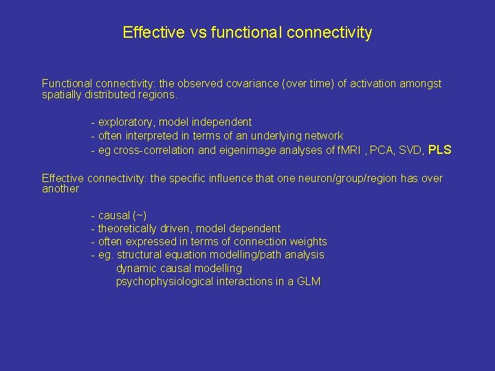
Effective vs functional connectivity Functional connectivity: the observed covariance (over time) of activation amongst spatially distributed regions. - exploratory, model independent - often interpreted in terms of an underlying network - eg cross-correlation and eigenimage analyses of f. MRI , PCA, SVD, PLS Effective connectivity: the specific influence that one neuron/group/region has over another - causal (~) - theoretically driven, model dependent - often expressed in terms of connection weights - eg. structural equation modelling/path analysis dynamic causal modelling psychophysiological interactions in a GLM

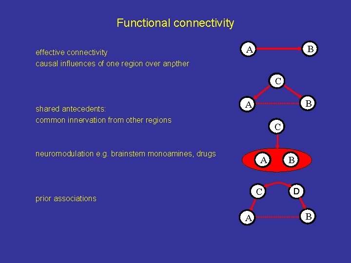
Functional connectivity effective connectivity causal influences of one region over another. B A C shared antecedents: common innervation from other regions B A C neuromodulation e. g. brainstem monoamines, drugs A C prior associations A B D B

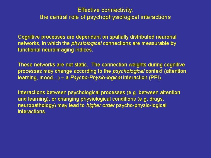
Effective connectivity: the central role of psychophysiological interactions Cognitive processes are dependant on spatially distributed neuronal networks, in which the physiological connections are measurable by functional neuroimaging indices. These networks are not static. The connection weights during cognitive processes may change according to the psychological context (attention, learning, mood…) – a Psycho-Physio-logical interaction (PPI). Interactions between psychological processes (e. g. between attention and learning), or changing physiological conditions (e. g. drugs, neuropathology) may lead to higher order psycho-physio-logical interactions.

Psychophysiological interactions (PPIs) Using PPIs, one gains experimental control over the network connectivity (mediating the task) AND the psychological or physiological contexts in which that task is performed. This enables the interpretation and understanding of the changes of effective connectivity in the proposed neural network. Different approaches to PPIs and effective connectivity 1. Using linear and non-linear terms as covariates in a GLM (PPI) 2. Structural equation modelling (SEM) 3. Dynamic causal modelling (DCM)

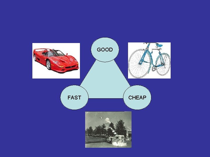
GOOD FAST CHEAP

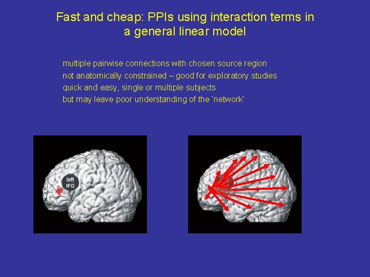
Fast and cheap: PPIs using interaction terms in a general linear model multiple pairwise connections with chosen source region not anatomically constrained – good for exploratory studies quick and easy, single or multiple subjects but may leave poor understanding of the ‘network’

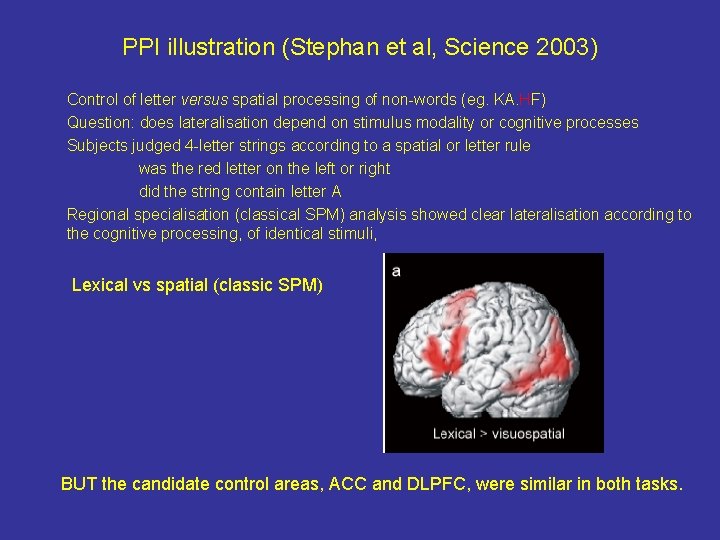
PPI illustration (Stephan et al, Science 2003) Control of letter versus spatial processing of non-words (eg. KA. HF) Question: does lateralisation depend on stimulus modality or cognitive processes Subjects judged 4 -letter strings according to a spatial or letter rule was the red letter on the left or right did the string contain letter A Regional specialisation (classical SPM) analysis showed clear lateralisation according to the cognitive processing, of identical stimuli, Lexical vs spatial (classic SPM) BUT the candidate control areas, ACC and DLPFC, were similar in both tasks.

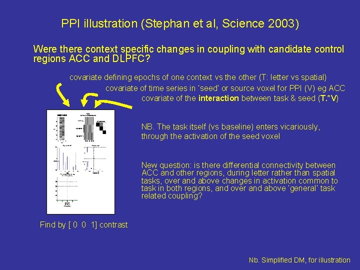
PPI illustration (Stephan et al, Science 2003) Were there context specific changes in coupling with candidate control regions ACC and DLPFC? covariate defining epochs of one context vs the other (T: letter vs spatial) covariate of time series in ‘seed’ or source voxel for PPI (V) eg ACC covariate of the interaction between task & seed (T. *V) NB. The task itself (vs baseline) enters vicariously, through the activation of the seed voxel New question: is there differential connectivity between ACC and other regions, during letter rather than spatial tasks, over and above changes in activation common to task in both regions, and over and above ‘general’ task related coupling? Find by [ 0 0 1] contrast Nb. Simplified DM, for illustration

SPM{t} of c=[ 0 0 1] from the interaction term: PPI of task x anterior cingulate Activation plot: IFG vs ACC, according to task Seed=ACC connectivity conclusion

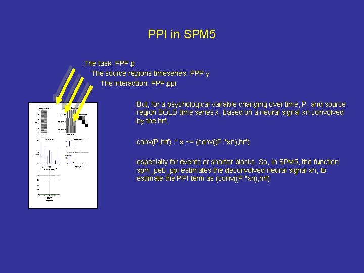
PPI in SPM 5. The task: PPP. p The source regions timeseries: PPP. y The interaction: PPP. ppi But, for a psychological variable changing over time, P, and source region BOLD time series x, based on a neural signal xn convolved by the hrf, conv(P, hrf). * x ~= (conv((P. *xn), hrf) especially for events or shorter blocks. So, in SPM 5, the function spm_peb_ppi estimates the deconvolved neural signal xn, to estimate the PPI term as (conv((P. *xn), hrf)

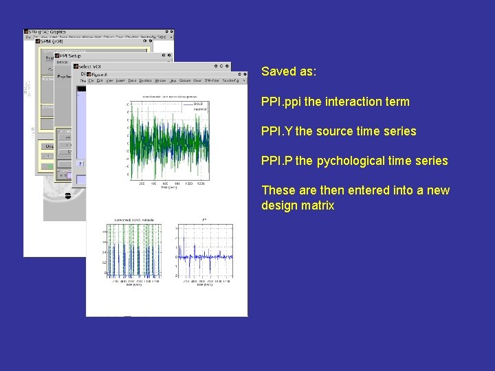
Saved as: PPI. ppi the interaction term PPI. Y the source time series PPI. P the pychological time series These are then entered into a new design matrix

SEM Theoretical framework introduced 1921 (Wright), developed in 1960’s for socioeconomics, and introduced to functional imaging 1990’s (Mc. Intosh, Gonzalez-Lima). 2. Easy to understand, fast to implement 3. PET and f. MRI applications, for single and multiple subjects 4. Complex networks ok – with care 4. It has specific advantages over other methods, including the ability to model multiple subjects simultaneously and test for inter-subject variance of connection strength directly.

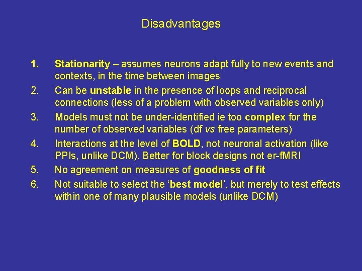
Disadvantages 1. 2. 3. 4. 5. 6. Stationarity – assumes neurons adapt fully to new events and contexts, in the time between images Can be unstable in the presence of loops and reciprocal connections (less of a problem with observed variables only) Models must not be under-identified ie too complex for the number of observed variables (df vs free parameters) Interactions at the level of BOLD, not neuronal activation (like PPIs, unlike DCM). Better for block designs not er-f. MRI No agreement on measures of goodness of fit Not suitable to select the ‘best model’, but merely to test effects within one of many plausible models (unlike DCM)

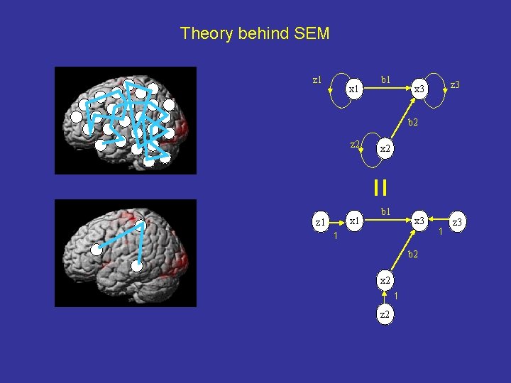
Theory behind SEM z 1 x 1 b 1 z 3 x 3 b 2 z 2 x 1 z 1 x 2 b 1 x 3 1 b 2 x 2 1 z 3

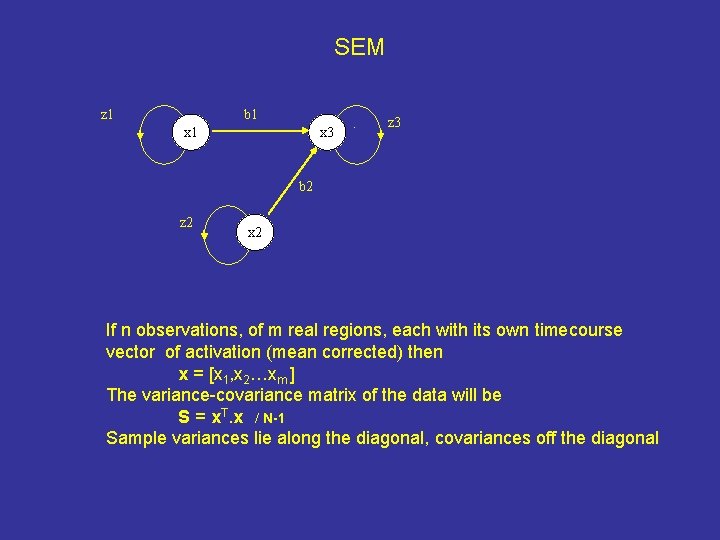
SEM z 1 b 1 x 3 . z 3 b 2 z 2 x 2 If n observations, of m real regions, each with its own timecourse vector of activation (mean corrected) then x = [x 1, x 2…xm ] The variance-covariance matrix of the data will be S = x. T. x / N-1 Sample variances lie along the diagonal, covariances off the diagonal

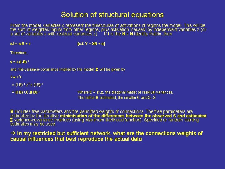
Solution of structural equations From the model, variables x represent the timecourse of activations of regions the model. This will be the sum of weighted inputs from other regions, plus activation ‘caused’ by independent variables z (or a set of variables x with residual variances z). If I is the N x N identity matrix, then x. I = x. B + z [c. f. Y = XB + e] Therefore, x = z. (I-B)-1 and, the variance-covariance implied by the model , S , will be given by S = x. Tx = (I-B)-1. z. T. z. (I-B)-1 = (I-B)-1. C. (I-B)-1 Where C = z. T. z, the diagonal matrix of residual variances, The better B estimated, the smaller C and S-S B includes free parameters and the permitted weights of connections. The free parameters are estimated by the iterative minimisation of the differences between the observed S and estimated S variance-covariance matrices (using Maximum likelihood function). Specified or random starting estimates may be used. In my restricted but sufficient network, what are the connections weights of causal influences that best reproduce the actual data

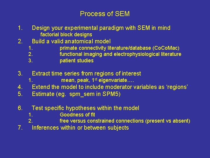
Process of SEM 1. Design your experimental paradigm with SEM in mind factorial block designs 2. Build a valid anatomical model 1. 2. 3. primate connectivity literature/database (Co. Mac) functional imaging and electrophysiological literature patient studies Extract time series from regions of interest 1. mean, peak, 1 st eigenvariate…. 4. 5. Extend the model to include moderator variables as ‘regions’ Estimate (eg. spm_sem in SPM 5) 6. Test specific hypotheses within the model 1. 2. 7. Goodness of fit free versus constrained connections (present vs absent) Inferences within or between subjects

Testing significance of path coefficients 1. 2. Single subject. Compare 2 (df=1) for two models in which a path is either permitted or omitted (set to 0). Between subjects. a. b. c. d. Determine the optimal parameters b 1 for a group of subjects one at a time, and test for b 1>0 using one sample ttest. Compare groups with unpaired t-tests for b 1 -g 1 ≠ b 1 -g 2 Put all subjects’ timeseries into one supermodel. Test as for 1. Build a single SEM, with all subjects, and compare 2 for the free model in which parameters for a path may vary between subjects, and a model in which the parameter is equal across all subjects. z 1 x 1 b 1 x 3 b 2 z 2 x 2 z 3

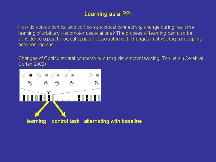
Learning as a PPI How do cortico-cortical and cortico-subcortical connectivity change during real time learning of arbitrary visuomotor associations? The process of learning can also be considered a psychological variable, associated with changes in physiological coupling between regions. covariance Changes of Cortico-striatal connectivity during visuomotor learning, Toni et al (Cerebral Cortex 2002). learning control task alternating with baseline

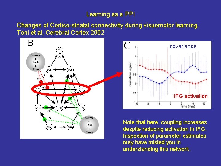
Learning as a PPI Changes of Cortico-striatal connectivity during visuomotor learning. Toni et al, Cerebral Cortex 2002 covariance IFG activation Note that here, coupling increases despite reducing activation in IFG. Inspection of parameter estimates may have misled you in understanding this network.

Pause. . Still to come: DCM

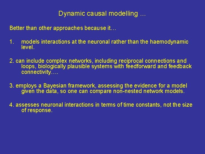
Dynamic causal modelling … Better than other approaches because it… 1. models interactions at the neuronal rather than the haemodynamic level. 2. can include complex networks, including reciprocal connections and loops, biologically plausible systems with feedforward and feedback connectivity…. 3. employs a Bayesian framework, assessing the evidence for a model given the data, so one can compare non-nested network models. 4. assesses neuronal interactions in terms of time constants, not the size of response.

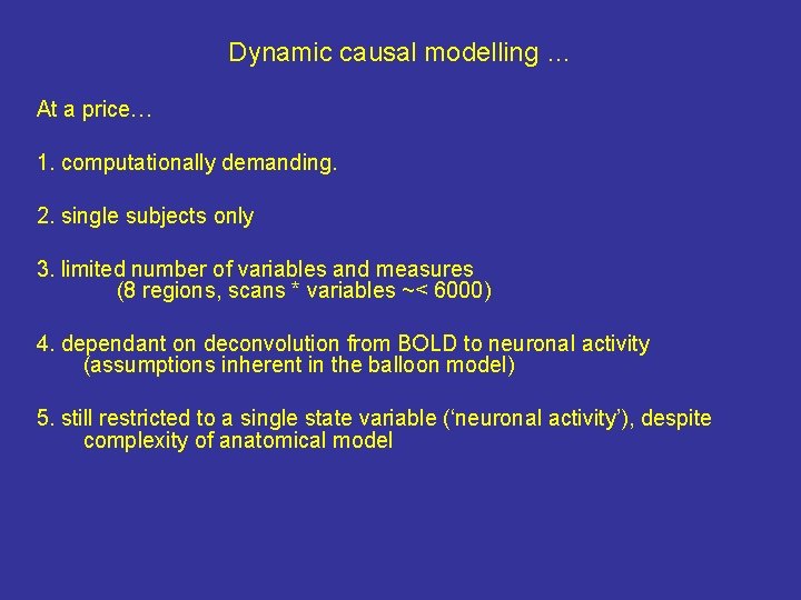
Dynamic causal modelling … At a price… 1. computationally demanding. 2. single subjects only 3. limited number of variables and measures (8 regions, scans * variables ~< 6000) 4. dependant on deconvolution from BOLD to neuronal activity (assumptions inherent in the balloon model) 5. still restricted to a single state variable (‘neuronal activity’), despite complexity of anatomical model

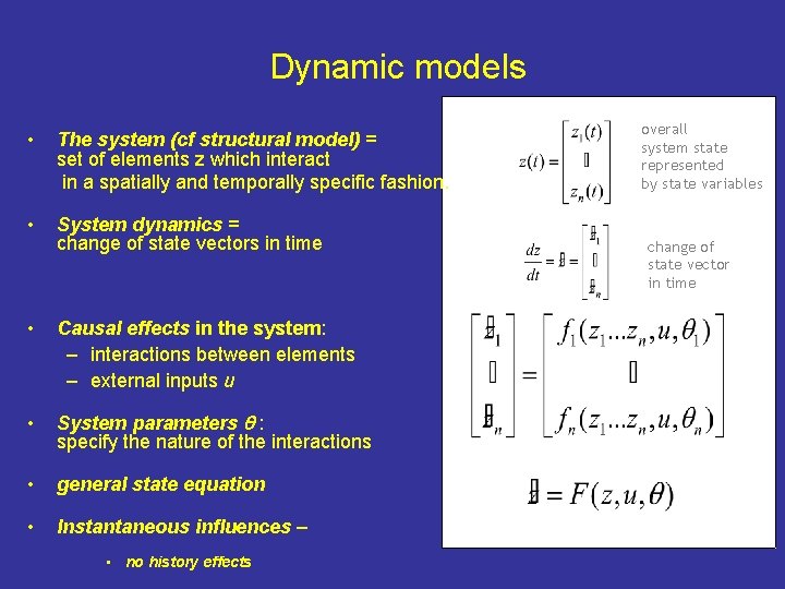
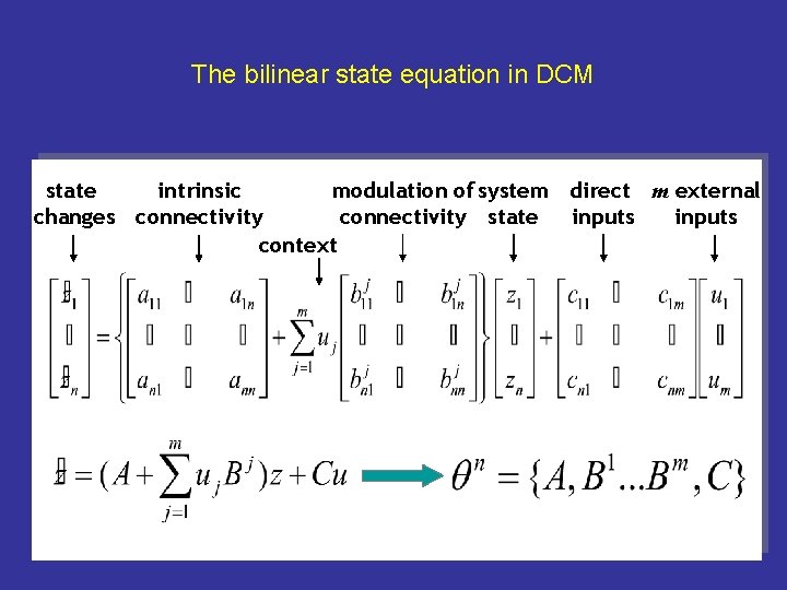
Dynamic models • The system (cf structural model) = set of elements z which interact in a spatially and temporally specific fashion. • System dynamics = change of state vectors in time • Causal effects in the system: – interactions between elements – external inputs u • System parameters : specify the nature of the interactions • general state equation • Instantaneous influences – • no history effects overall system state represented by state variables change of state vector in time

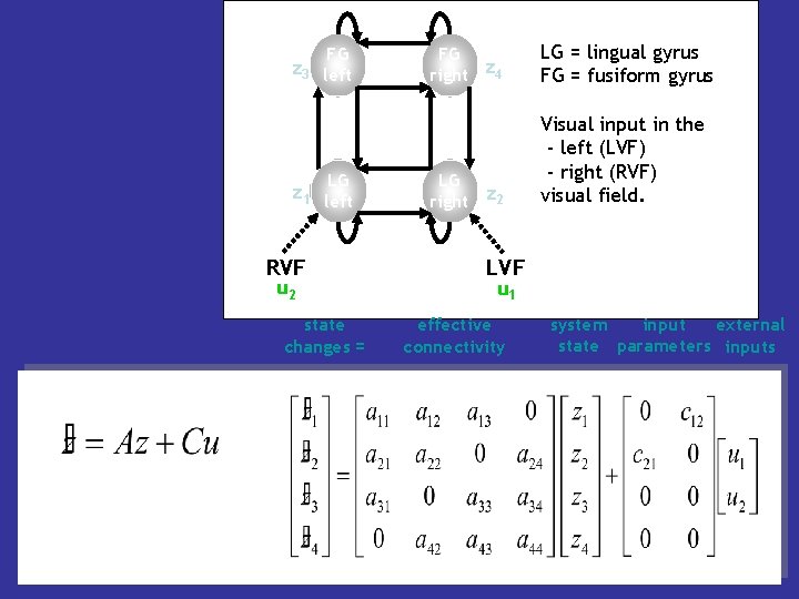
FG z 3 left LG z 1 left RVF u 2 state changes = FG right z 4 LG = lingual gyrus FG = fusiform gyrus LG right z 2 Visual input in the - left (LVF) - right (RVF) visual field. LVF u 1 effective connectivity system input external state parameters inputs

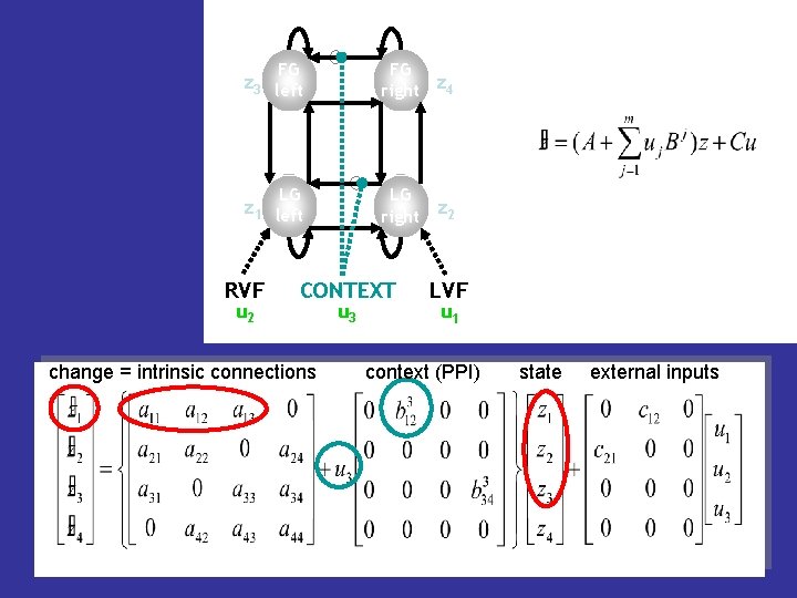
z 3 FG left FG right z 4 LG LG right z 2 z 1 left RVF u 2 CONTEXT u 3 LVF u 1 change = intrinsic connections context (PPI) state external inputs

The bilinear state equation in DCM modulation of system direct m external state intrinsic connectivity state inputs changes connectivity inputs context

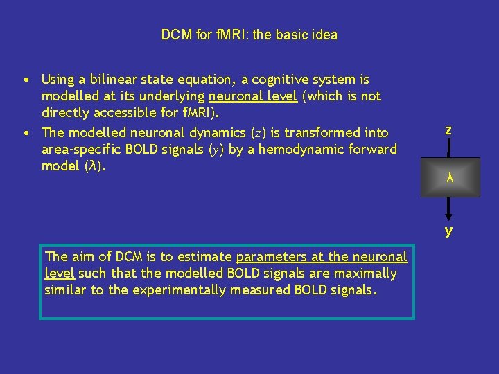
DCM for f. MRI: the basic idea • Using a bilinear state equation, a cognitive system is modelled at its underlying neuronal level (which is not directly accessible for f. MRI). • The modelled neuronal dynamics (z) is transformed into area-specific BOLD signals (y) by a hemodynamic forward model (λ). z λ y The aim of DCM is to estimate parameters at the neuronal level such that the modelled BOLD signals are maximally similar to the experimentally measured BOLD signals.

The haemodynamic “Balloon” model • 5 haemodynamic parameters: important for model fitting, but of no interest for statistical inference • Empirically determined a priori distributions. • Computed separately for each area (like the neural parameters).

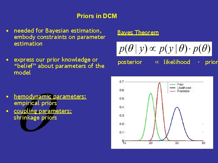
Priors in DCM • needed for Bayesian estimation, embody constraints on parameter estimation Bayes Theorem • express our prior knowledge or “belief” about parameters of the model posterior • hemodynamic parameters: empirical priors • coupling parameters: shrinkage priors likelihood ∙ prior

Inference about DCM parameters: Bayesian single-subject analysis • Bayesian parameter estimation in DCM: Gaussian assumptions about the posterior distributions of the parameters • SPM-DCM uses the cumulative normal distribution to test the probability by which a certain parameter is above a chosen threshold γ: • γ can be chosen as zero ("does the effect exist? ") or as a function of the expected half life τ of the neural process: γ = ln 2 / τ

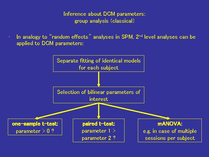
Inference about DCM parameters: group analysis (classical) • In analogy to “random effects” analyses in SPM, 2 nd level analyses can be applied to DCM parameters: Separate fitting of identical models for each subject Selection of bilinear parameters of interest one-sample t-test: parameter > 0 ? paired t-test: parameter 1 > parameter 2 ? m. ANOVA: e. g. in case of multiple sessions per subject

Planning a DCM-compatible study • Suitable experimental design: – preferably factorial (e. g. 2 x 2) – with one factor that varies the driving (sensory) input – and one factor that varies the contextual input (cf PPI) • TR: – as short as possible (optimal: < 2 s) • Hypothesis driven and again model dependent: – define specific a priori hypothesis – which parameters are relevant to test this hypothesis? – ensure that intended model is suitable to test this hypothesis → simulations before experiment – define method and criteria for statistics and inference

Practical steps of a DCM study - I 1. Conventional SPM analysis (subject-specific) • DCMs are fitted separately for each session → consider concatenation of sessions or if adequate, a 2 nd level analysis 2. Definition of the model (on paper!) • Structure: which areas, connections and inputs? • Which parameters represent my hypothesis? • How can I demonstrate the specificity of my results? • What are the alternative models to test? 3. Defining criteria for inference: • single-subject analysis: • group analysis: threshold? contrast? which 2 nd-level model?

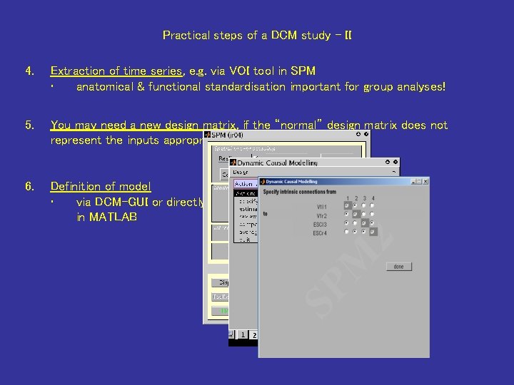
Practical steps of a DCM study - II 4. Extraction of time series, e. g. via VOI tool in SPM • anatomical & functional standardisation important for group analyses! 5. You may need a new design matrix, if the “normal” design matrix does not represent the inputs appropriately. 6. Definition of model • via DCM-GUI or directly in MATLAB

Practical steps of a DCM study - III 7. DCM parameter estimation • note: models with many regions & scans can crash MATLAB! 8. Model comparison and selection: • Which of all models considered is the optimal one? Bayesian model comparison tool 9. Testing the hypothesis Statistical test on the relevant parameters of the optimal model

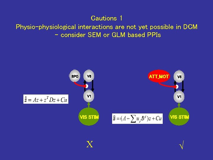
Cautions 1 Physio-physiological interactions are not yet possible in DCM - consider SEM or GLM based PPIs SPC V 5 ATT_MOT V 5 V 1 VIS STIM X √

Cautions 2 DCM_group_average is not the average of a group of DCMs! Having completed a set of first level subject specific DCMs, you now want to summarise the group Do you: a. perform standard parametric tests (ANOVAs, 1 -sapmple t-tests etc) to the connection parameters (Hz) like for SEMs or SPMs? b. Use spm_dcm_average? c. d. There are quite a few messages discussing this on the SPM list, but I suggest using dcm_average, with caution. It does not take the arithmetic mean of the first level parameters. Rather it rolls through the group using the values of previous subject(s) as priors for the next subject. Values are weighted according to the first level precision (inverse of variance)…

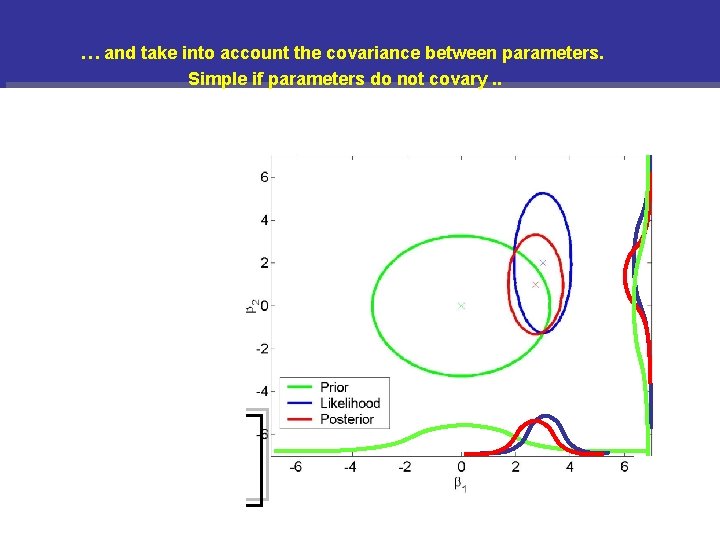
. … and take into account the covariance between parameters. Simple if parameters do not covary. . Normal densities

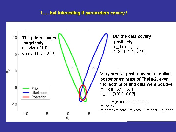
. 1. … but interesting if parameters covary !. The priors covary negatively m_prior = [1, 1] σ_prior-[1 -3 ; -3 10] But the data covary positively m_data = [6, 1] σ_prior-[1 3 ; 3 10] Very precise posteriors but negative posterior estimate of Theta-2, even tho’ both prior and data were positive m_post=[3. 5 -6. 5] σ_post=[0. 05 0 ; 0 0. 5] σ_post = (σ_data-1+ σ_prior-1)-1 m_post = σ_post * (σ_data-1*m_data + σ_prior-1*m_prior)

Summary Effective connectivity Hypothesis driven, model dependant Concept of psychophysiological interactions Specific methods: PPI in GLM, SEM, DCM Further reading: Karl Friston, Will Penny, Klaas Stephan SPM list and SPM pages www. fil. ion. ucl. ac. uk/spm

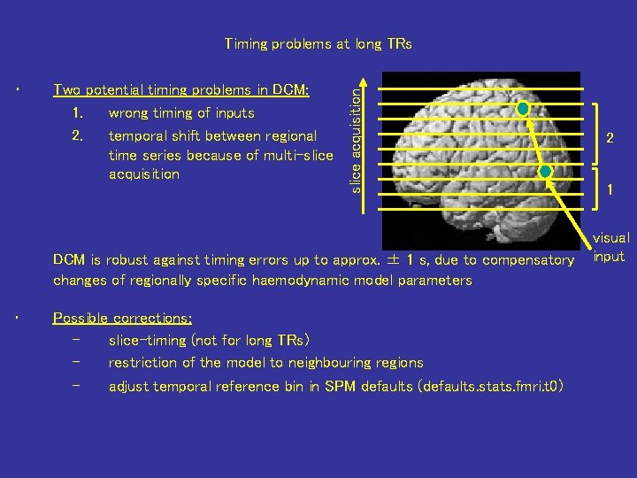
• Two potential timing problems in DCM: 1. wrong timing of inputs 2. temporal shift between regional time series because of multi-slice acquisition Timing problems at long TRs DCM is robust against timing errors up to approx. ± 1 s, due to compensatory changes of regionally specific haemodynamic model parameters • Possible corrections: – slice-timing (not for long TRs) – restriction of the model to neighbouring regions – adjust temporal reference bin in SPM defaults (defaults. stats. fmri. t 0) 2 1 visual input

Model comparison and selection Pitt & Miyung (2002), TICS Akaike information criterion (AIC) and Bayesian information criterion (BIC): Assess evidence in terms of accuracy of a model given its complexity.

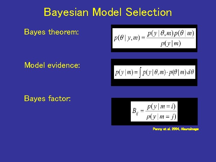
Bayesian Model Selection Bayes theorem: Model evidence: Bayes factor: Penny et al. 2004, Neuro. Image

illustration covariance path analysis (partial correlation) A r=0. 48 ~0. 5 B A r=0. 29 ~0. 3 r=0. 15 ~0. 15 a=BOLD 200 b=0. 5 a+0. 5 noise c=0. 3 a+0. 7 noise C p=0. 48 ~0. 5 B p=0. 29 ~0. 3 p=0. 01 ~0. 0 C

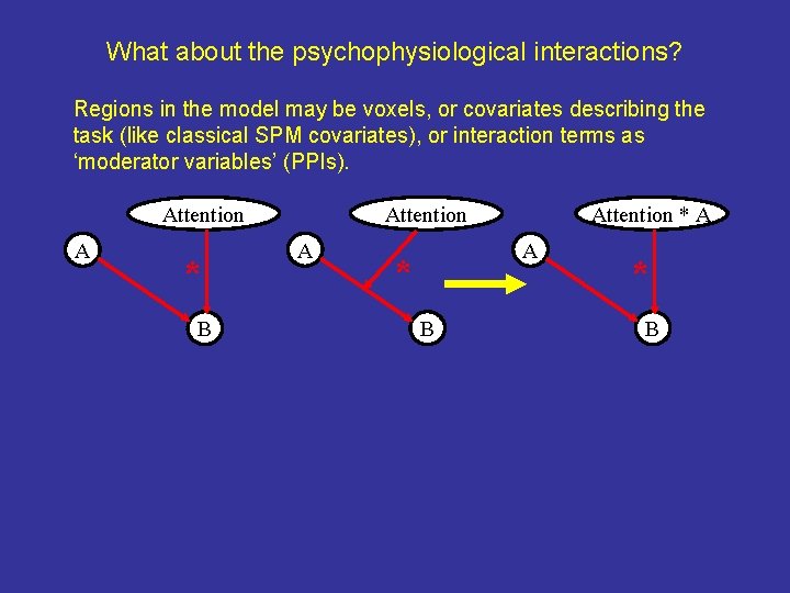
What about the psychophysiological interactions? Regions in the model may be voxels, or covariates describing the task (like classical SPM covariates), or interaction terms as ‘moderator variables’ (PPIs). Attention A * B Attention A Attention * A A * B

DATA structures (stacking models) SEM in SPM [C, B, 2, df] Model design/complexity g) n i t es n ( B bles n o ia s r n a o v i ict rator r t s Re ode m inc

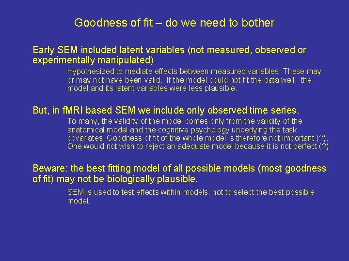
Goodness of fit – do we need to bother Early SEM included latent variables (not measured, observed or experimentally manipulated) Hypothesized to mediate effects between measured variables. These may or may not have been valid. If the model could not fit the data well, the model and its latent variables were less plausible. But, in f. MRI based SEM we include only observed time series. To many, the validity of the model comes only from the validity of the anatomical model and the cognitive psychology underlying the task covariates. Goodness of fit of the whole model is therefore not important (? ). One would not wish to reject an adequate model because it is not perfect (? ) Beware: the best fitting model of all possible models (most goodness of fit) may not be biologically plausible. SEM is used to test effects within models, not to select the best possible model.

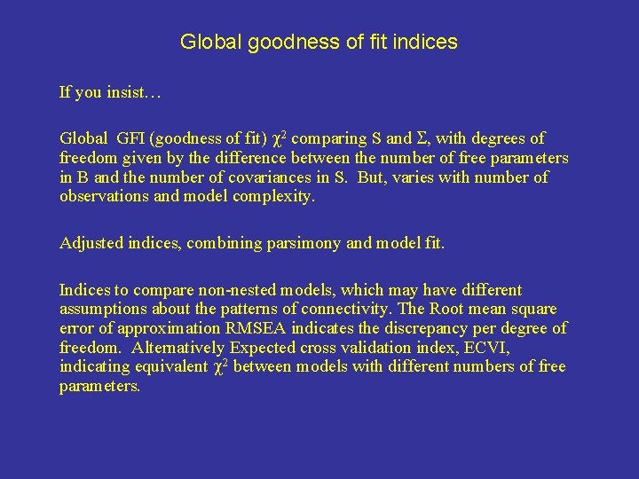
Global goodness of fit indices If you insist… Global GFI (goodness of fit) 2 comparing S and S, with degrees of freedom given by the difference between the number of free parameters in B and the number of covariances in S. But, varies with number of observations and model complexity. Adjusted indices, combining parsimony and model fit. Indices to compare non-nested models, which may have different assumptions about the patterns of connectivity. The Root mean square error of approximation RMSEA indicates the discrepancy per degree of freedom. Alternatively Expected cross validation index, ECVI, indicating equivalent 2 between models with different numbers of free parameters.

Questions .