Analysis of continuous surfaces filtering slopes shading Peter

Analysis of ‘continuous surfaces’ (filtering, slopes, shading) Peter Fox GIS for Science ERTH 4750 (98271) Week 7, Tuesday, March 6, 2012 1

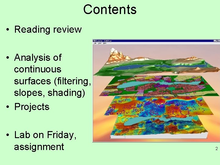
Contents • Reading review • Analysis of continuous surfaces (filtering, slopes, shading) • Projects • Lab on Friday, assignment 2

Reading for last week • • • Geostatistics References Kriging (wikipedia) Bohling on Kriging Bohling on Variograms Query – Help with SQL (Standard Query Language) – Chapter 8 in Map. Info User Guide (10. 5): Selecting and Querying Data (p. 193 -228) 3

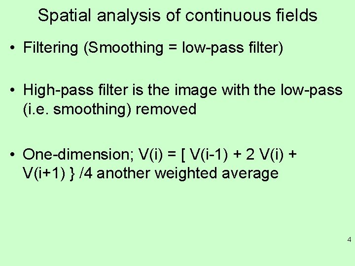
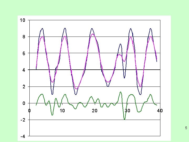
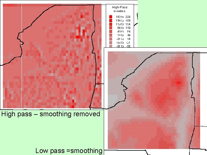
Spatial analysis of continuous fields • Filtering (Smoothing = low-pass filter) • High-pass filter is the image with the low-pass (i. e. smoothing) removed • One-dimension; V(i) = [ V(i-1) + 2 V(i) + V(i+1) } /4 another weighted average 4

5

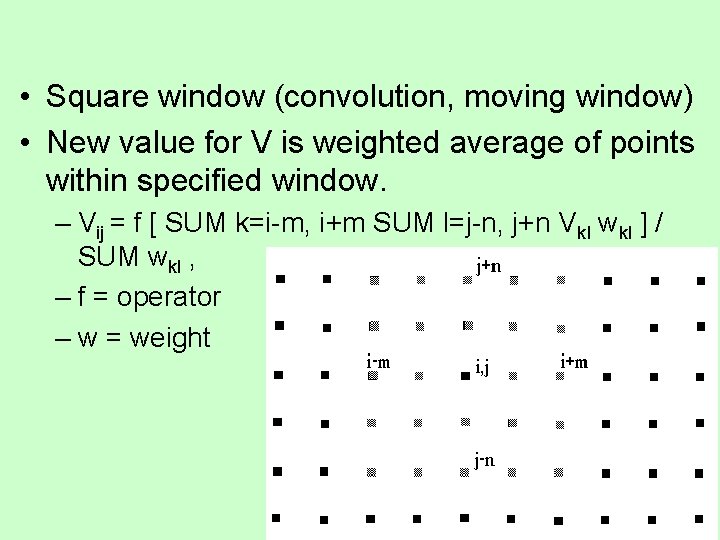
• Square window (convolution, moving window) • New value for V is weighted average of points within specified window. – Vij = f [ SUM k=i-m, i+m SUM l=j-n, j+n Vkl wkl ] / SUM wkl , – f = operator – w = weight 6

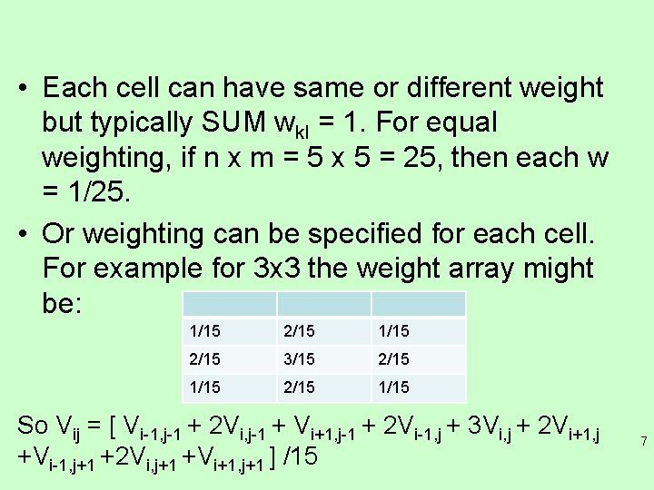
• Each cell can have same or different weight but typically SUM wkl = 1. For equal weighting, if n x m = 5 x 5 = 25, then each w = 1/25. • Or weighting can be specified for each cell. For example for 3 x 3 the weight array might be: 1/15 2/15 3/15 2/15 1/15 So Vij = [ Vi-1, j-1 + 2 Vi, j-1 + Vi+1, j-1 + 2 Vi-1, j + 3 Vi, j + 2 Vi+1, j +Vi-1, j+1 +2 Vi, j+1 +Vi+1, j+1 ] /15 7

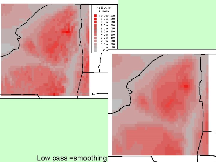
8 Low pass =smoothing

High pass – smoothing removed 9 Low pass =smoothing

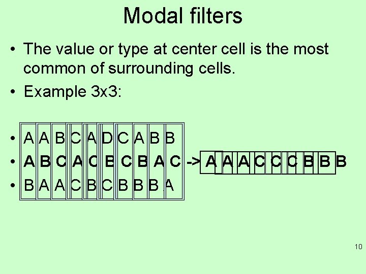
Modal filters • The value or type at center cell is the most common of surrounding cells. • Example 3 x 3: • AABCADCABB • A B C A C B A C -> A A A C C C B B B • BAACBCBBBA 10

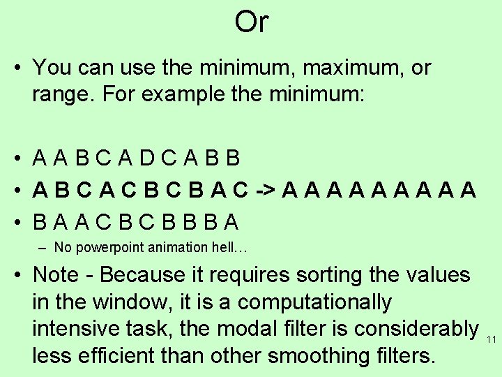
Or • You can use the minimum, maximum, or range. For example the minimum: • AABCADCABB • A B C A C B A C -> A A A A A • BAACBCBBBA – No powerpoint animation hell… • Note - Because it requires sorting the values in the window, it is a computationally intensive task, the modal filter is considerably 11 less efficient than other smoothing filters.

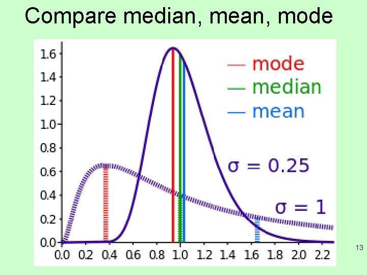
Median filter • Median filters can be used to emphasize the longerrange variability in an image, effectively acting to smooth the image. • This can be useful for reducing the noise in an image. The algorithm operates by calculating the median value (middle value in a sorted list) in a moving window centered on each grid cell. • The median value is not influenced by anomalously high or low values in the distribution to the extent that the average is. • As such, the median filter is far less sensitive to shot 12 noise in an image than the mean filter.

Compare median, mean, mode 13

Median filter • Because it requires sorting the values in the window, a computationally intensive task, the median filter is considerably less efficient than other smoothing filters. • This may pose a problem for large images or large neighborhoods. • Neighborhood size, or filter size, is determined by the userdefined x and y dimensions. These dimensions should be odd, positive integer values, e. g. 3, 5, 7, 9. . . • You may also define the neighborhood shape as either squared or rounded. • A rounded neighborhood approximates an ellipse; a rounded neighborhood with equal x and y dimensions approximates a 14 circle.

Sobel filter • Edge detection – performs a 3 x 3 or 5 x 5 Sobel edge-detection filter on a raster image. • The Sobel filter is similar to the Prewitt filter, in that it identifies areas of high slope in the input image through the calculation of slopes in the x and y directions. • The Sobel edge-detection filter, however, gives more weight to nearer cell values within the moving window, or kernel. 15

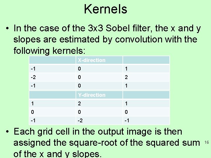
Kernels • In the case of the 3 x 3 Sobel filter, the x and y slopes are estimated by convolution with the following kernels: X-direction -1 0 1 -2 0 2 -1 0 1 Y-direction 1 2 1 0 0 0 -1 -2 -1 • Each grid cell in the output image is then assigned the square-root of the squared sum of the x and y slopes. 16

Reading – Spatial Filters • Do some web searches • What about temporal filtering ? ? ? – Trick question 17

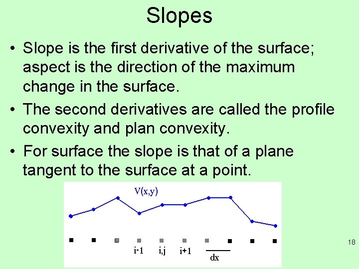
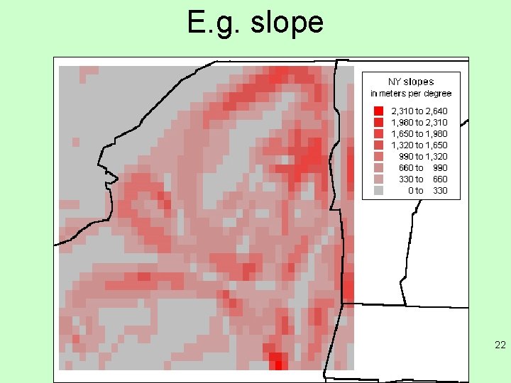
Slopes • Slope is the first derivative of the surface; aspect is the direction of the maximum change in the surface. • The second derivatives are called the profile convexity and plan convexity. • For surface the slope is that of a plane tangent to the surface at a point. 18

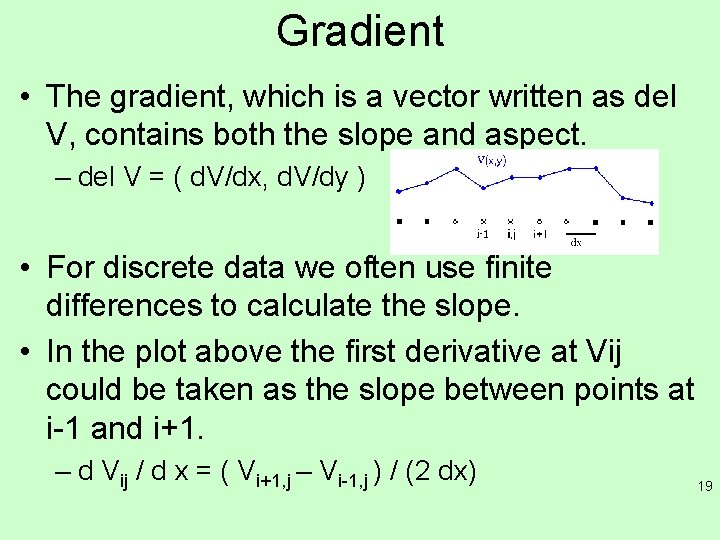
Gradient • The gradient, which is a vector written as del V, contains both the slope and aspect. – del V = ( d. V/dx, d. V/dy ) • For discrete data we often use finite differences to calculate the slope. • In the plot above the first derivative at Vij could be taken as the slope between points at i-1 and i+1. – d Vij / d x = ( Vi+1, j – Vi-1, j ) / (2 dx) 19

Second derivative • … is the slope of the slope. We take the change in slope between i+1 and i, and between i and i-1. d 2 V / dx 2 = [ ( Vi+1, j – Vi, j ) / dx - ( Vi, j – Vi-1, j ) / dx ] / dx • The slope, which is the magnitude of del V, is: | del V | = [ (d V / d x )2 + ( d V / d y )2 ]1/2 20

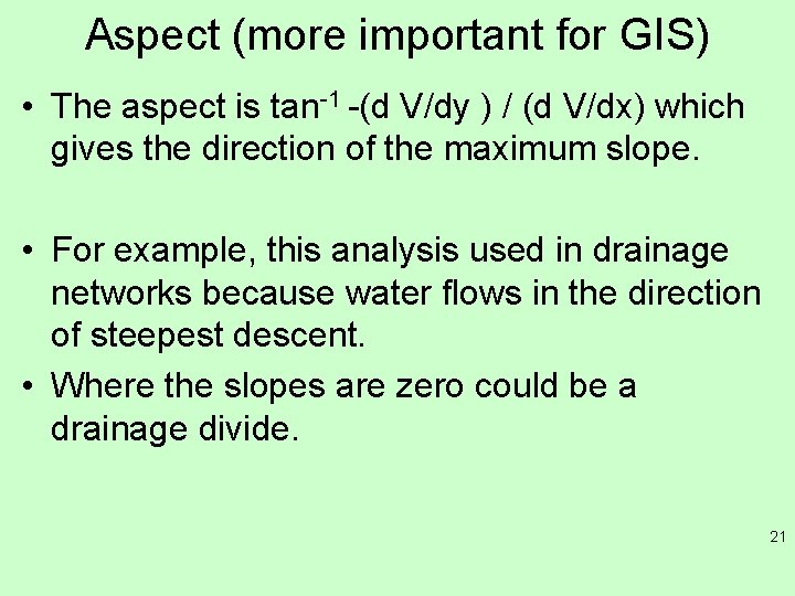
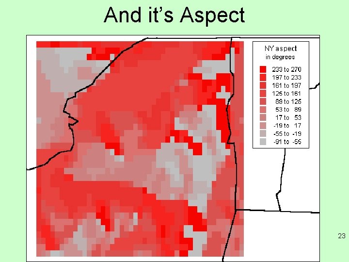
Aspect (more important for GIS) • The aspect is tan-1 -(d V/dy ) / (d V/dx) which gives the direction of the maximum slope. • For example, this analysis used in drainage networks because water flows in the direction of steepest descent. • Where the slopes are zero could be a drainage divide. 21

E. g. slope 22

And it’s Aspect 23

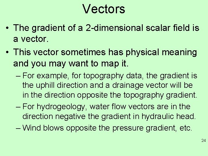
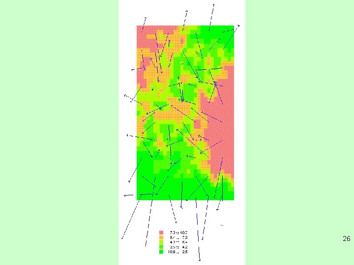
Vectors • The gradient of a 2 -dimensional scalar field is a vector. • This vector sometimes has physical meaning and you may want to map it. – For example, for topography data, the gradient is the uphill direction and a drainage vector will be in the direction opposite the topography gradient. – For hydrogeology, water flow vectors are in the direction negative the gradient in hydraulic head. – Wind blows opposite the pressure gradient, etc. 24

Ah-Map. Info has a cousin • Map. Info does not directly let you plot vectors but you can do this fairly easily with Map. Basic. • Since the x-component of the gradient is d. V/dx and the y-component is d. V/dy, you can build a line object that starts at the grid point (X, Y) and ends at the point (X + d. V/dx, Y + d. V/dy) (some scaling is required and you choose the arrow option for the line type). 25

26

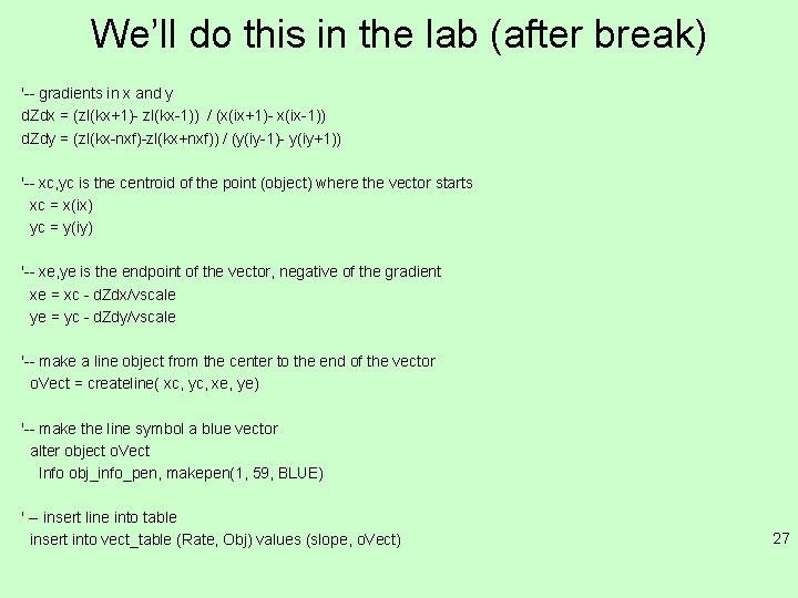
We’ll do this in the lab (after break) '-- gradients in x and y d. Zdx = (zl(kx+1)- zl(kx-1)) / (x(ix+1)- x(ix-1)) d. Zdy = (zl(kx-nxf)-zl(kx+nxf)) / (y(iy-1)- y(iy+1)) '-- xc, yc is the centroid of the point (object) where the vector starts xc = x(ix) yc = y(iy) '-- xe, ye is the endpoint of the vector, negative of the gradient xe = xc - d. Zdx/vscale ye = yc - d. Zdy/vscale '-- make a line object from the center to the end of the vector o. Vect = createline( xc, yc, xe, ye) '-- make the line symbol a blue vector alter object o. Vect Info obj_info_pen, makepen(1, 59, BLUE) ' -- insert line into table insert into vect_table (Rate, Obj) values (slope, o. Vect) 27

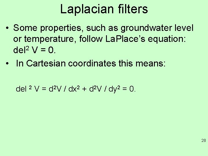
Laplacian filters • Some properties, such as groundwater level or temperature, follow La. Place’s equation: del 2 V = 0. • In Cartesian coordinates this means: del 2 V = d 2 V / dx 2 + d 2 V / dy 2 = 0. 28

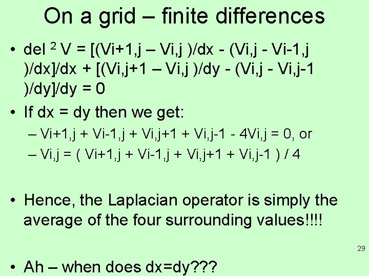
On a grid – finite differences • del 2 V = [(Vi+1, j – Vi, j )/dx - (Vi, j - Vi-1, j )/dx]/dx + [(Vi, j+1 – Vi, j )/dy - (Vi, j - Vi, j-1 )/dy]/dy = 0 • If dx = dy then we get: – Vi+1, j + Vi-1, j + Vi, j+1 + Vi, j-1 - 4 Vi, j = 0, or – Vi, j = ( Vi+1, j + Vi-1, j + Vi, j+1 + Vi, j-1 ) / 4 • Hence, the Laplacian operator is simply the average of the four surrounding values!!!! 29 • Ah – when does dx=dy? ? ?

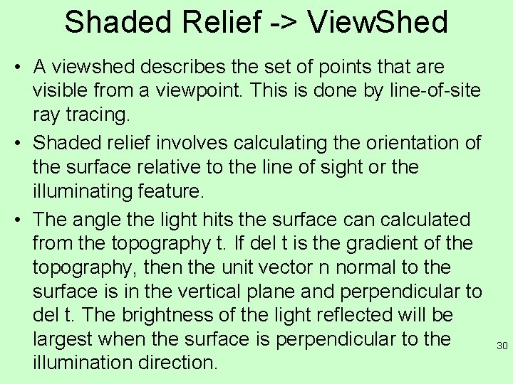
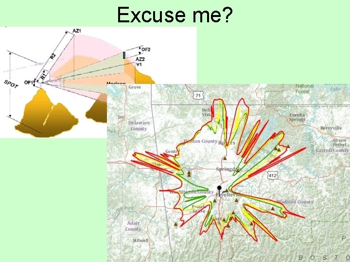
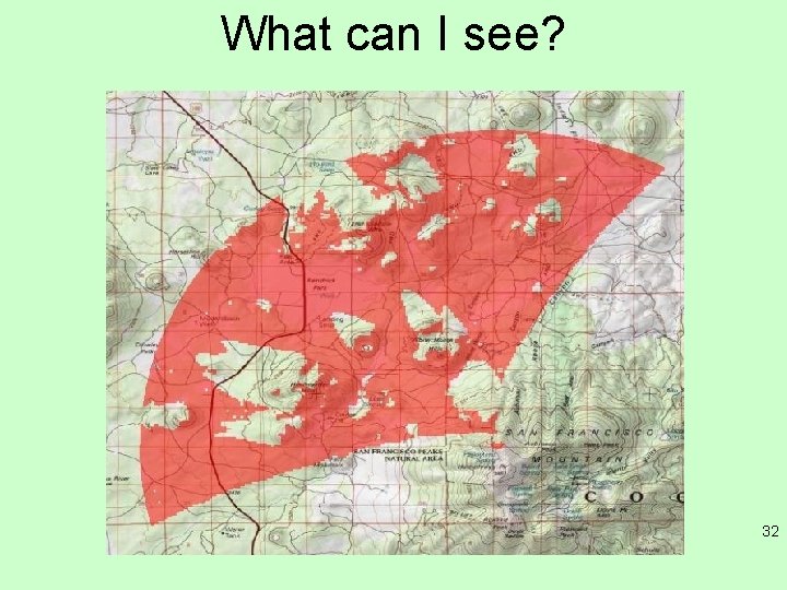
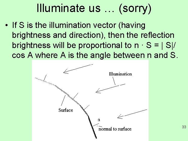
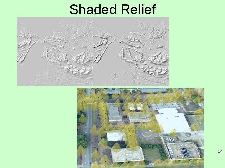
Shaded Relief -> View. Shed • A viewshed describes the set of points that are visible from a viewpoint. This is done by line-of-site ray tracing. • Shaded relief involves calculating the orientation of the surface relative to the line of sight or the illuminating feature. • The angle the light hits the surface can calculated from the topography t. If del t is the gradient of the topography, then the unit vector n normal to the surface is in the vertical plane and perpendicular to del t. The brightness of the light reflected will be largest when the surface is perpendicular to the illumination direction. 30

Excuse me? 31

What can I see? 32

Illuminate us … (sorry) • If S is the illumination vector (having brightness and direction), then the reflection brightness will be proportional to n · S = | S|/ cos A where A is the angle between n and S. 33

Shaded Relief 34

Summary • Topics for GIS (for Science) – Filtering, slopes + , enhancements • For learning purposes remember: – Demonstrate proficiency in using geospatial applications and tools (commercial and open-source). – Present verbally relational analysis and interpretation of a variety of spatial data on maps. – Demonstrate skill in applying database concepts to build and manipulate a spatial database, SQL, spatial queries, and integration of graphic and tabular data. – Demonstrate intermediate knowledge of geospatial analysis methods and their applications. 35

Friday Mar. 9 • Lab assignment session – two problems, I’ll put them up right after class today • Complete them in class, get signed off before leaving • 10% of grade 36

Reading for this week • NONE!! Happy spring break 37

Next classes • Tuesday, March 20, Analysis of errors • Friday, March 23 – lab with material from this week (lab assignment 10%) • Note March 30 – open lab (no assignment, work on projects, get help from Max) 38