Analysis of Algorithms CS 477677 Dynamic Programming Instructor

Analysis of Algorithms CS 477/677 Dynamic Programming Instructor: George Bebis (Chapter 15) CS 465/665 - Lecture 14

Dynamic Programming • An algorithm design technique (like divide and conquer) • Divide and conquer – Partition the problem into independent subproblems – Solve the subproblems recursively – Combine the solutions to solve the original problem 2

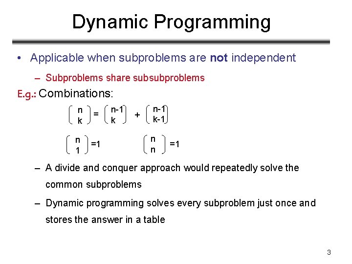
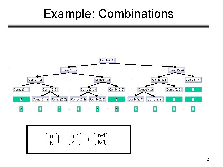
Dynamic Programming • Applicable when subproblems are not independent – Subproblems share subsubproblems E. g. : Combinations: n k = n 1 =1 n-1 k + n-1 k-1 n n =1 – A divide and conquer approach would repeatedly solve the common subproblems – Dynamic programming solves every subproblem just once and stores the answer in a table 3

Example: Combinations n k = n-1 k + n-1 k-1 4

Dynamic Programming • Used for optimization problems – A set of choices must be made to get an optimal solution – Find a solution with the optimal value (minimum or maximum) – There may be many solutions that lead to an optimal value – Our goal: find an optimal solution 5

Dynamic Programming Algorithm 1. Characterize the structure of an optimal solution 2. Recursively define the value of an optimal solution 3. Compute the value of an optimal solution in a bottom-up fashion 4. Construct an optimal solution from computed information (not always necessary) 6

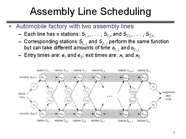
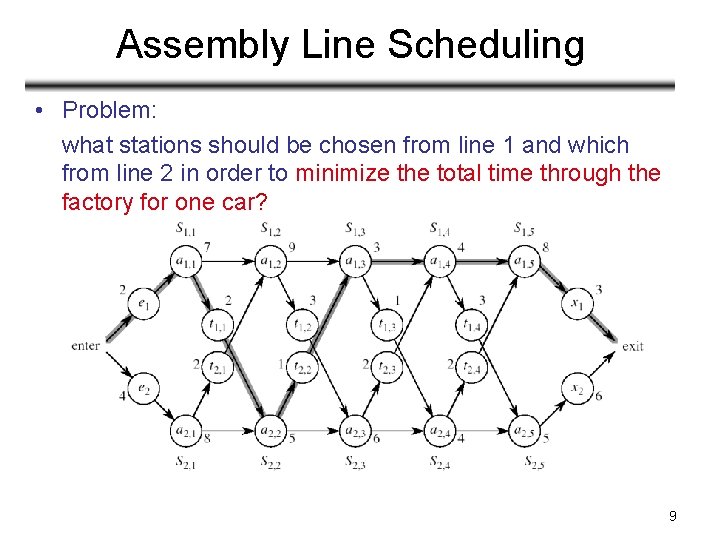
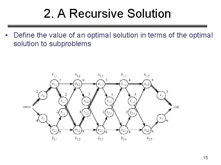
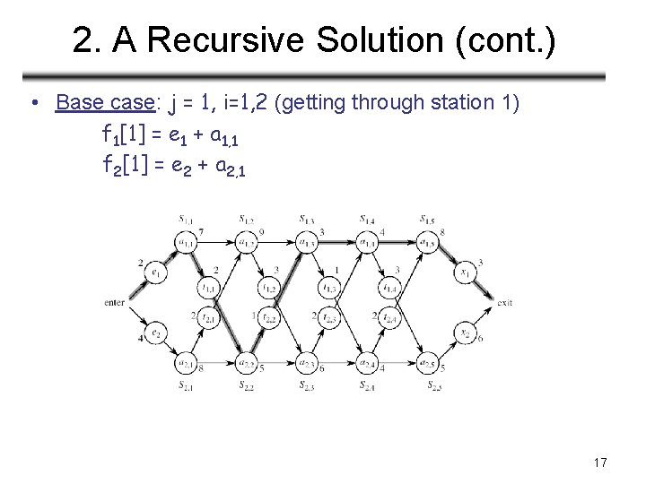
Assembly Line Scheduling • Automobile factory with two assembly lines – Each line has n stations: S 1, 1, . . . , S 1, n and S 2, 1, . . . , S 2, n – Corresponding stations S 1, j and S 2, j perform the same function but can take different amounts of time a 1, j and a 2, j – Entry times are: e 1 and e 2; exit times are: x 1 and x 2 7

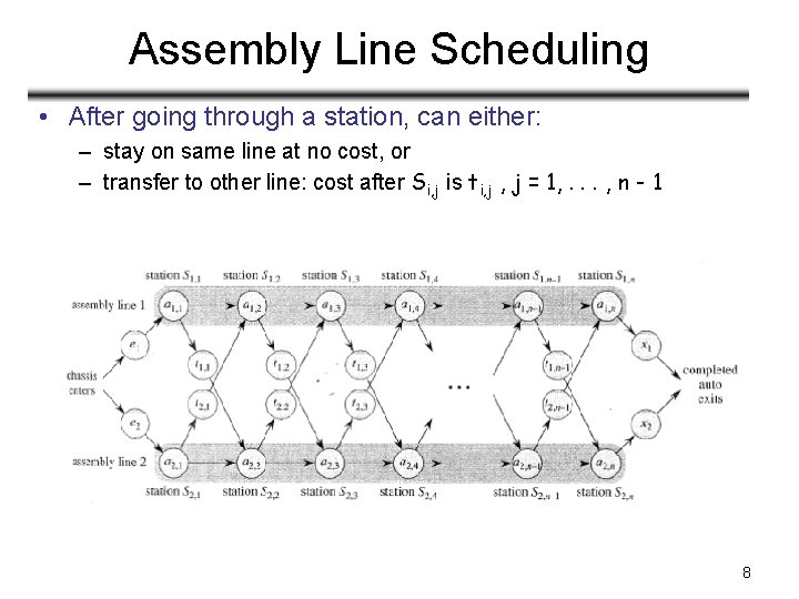
Assembly Line Scheduling • After going through a station, can either: – stay on same line at no cost, or – transfer to other line: cost after Si, j is ti, j = 1, . . . , n - 1 8

Assembly Line Scheduling • Problem: what stations should be chosen from line 1 and which from line 2 in order to minimize the total time through the factory for one car? 9

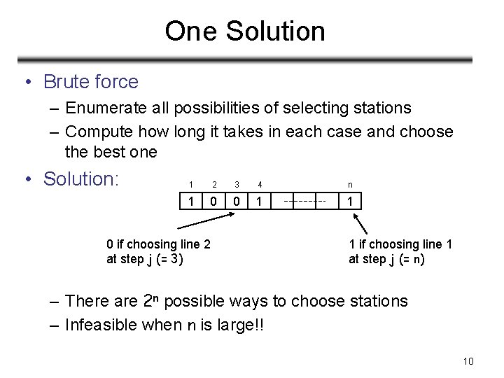
One Solution • Brute force – Enumerate all possibilities of selecting stations – Compute how long it takes in each case and choose the best one • Solution: 1 2 3 4 n 1 0 0 1 1 0 if choosing line 2 at step j (= 3) 1 if choosing line 1 at step j (= n) – There are 2 n possible ways to choose stations – Infeasible when n is large!! 10

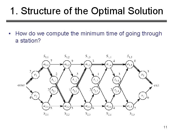
1. Structure of the Optimal Solution • How do we compute the minimum time of going through a station? 11

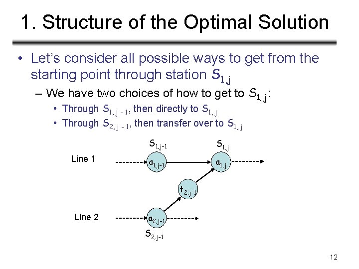
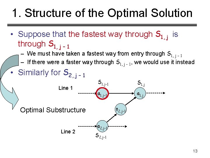
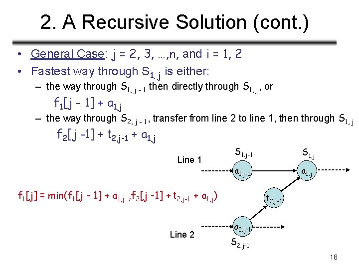
1. Structure of the Optimal Solution • Let’s consider all possible ways to get from the starting point through station S 1, j – We have two choices of how to get to S 1, j: • Through S 1, j - 1, then directly to S 1, j • Through S 2, j - 1, then transfer over to S 1, j Line 1 S 1, j-1 S 1, j a 1, j-1 a 1, j t 2, j-1 Line 2 a 2, j-1 S 2, j-1 12

1. Structure of the Optimal Solution • Suppose that the fastest way through S 1, j is through S 1, j – 1 – We must have taken a fastest way from entry through S 1, j – 1 – If there were a faster way through S 1, j - 1, we would use it instead • Similarly for S 2, j – 1 Line 1 S 1, j-1 S 1, j a 1, j-1 a 1, j t 2, j-1 Optimal Substructure Line 2 a 2, j-1 S 2, j-1 13

Optimal Substructure • Generalization: an optimal solution to the problem “find the fastest way through S 1, j” contains within it an optimal solution to subproblems: “find the fastest way through S 1, j - 1 or S 2, j – 1”. • This is referred to as the optimal substructure property • We use this property to construct an optimal solution to a problem from optimal solutions to subproblems 14

2. A Recursive Solution • Define the value of an optimal solution in terms of the optimal solution to subproblems 15

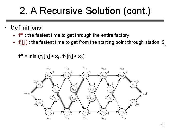
2. A Recursive Solution (cont. ) • Definitions: – f* : the fastest time to get through the entire factory – fi[j] : the fastest time to get from the starting point through station Si, j f* = min (f 1[n] + x 1, f 2[n] + x 2) 16

2. A Recursive Solution (cont. ) • Base case: j = 1, i=1, 2 (getting through station 1) f 1[1] = e 1 + a 1, 1 f 2[1] = e 2 + a 2, 1 17

2. A Recursive Solution (cont. ) • General Case: j = 2, 3, …, n, and i = 1, 2 • Fastest way through S 1, j is either: – the way through S 1, j - 1 then directly through S 1, j, or f 1[j - 1] + a 1, j – the way through S 2, j - 1, transfer from line 2 to line 1, then through S 1, j f 2[j -1] + t 2, j-1 + a 1, j Line 1 S 1, j-1 S 1, j a 1, j-1 a 1, j f 1[j] = min(f 1[j - 1] + a 1, j , f 2[j -1] + t 2, j-1 + a 1, j) Line 2 t 2, j-1 a 2, j-1 S 2, j-1 18

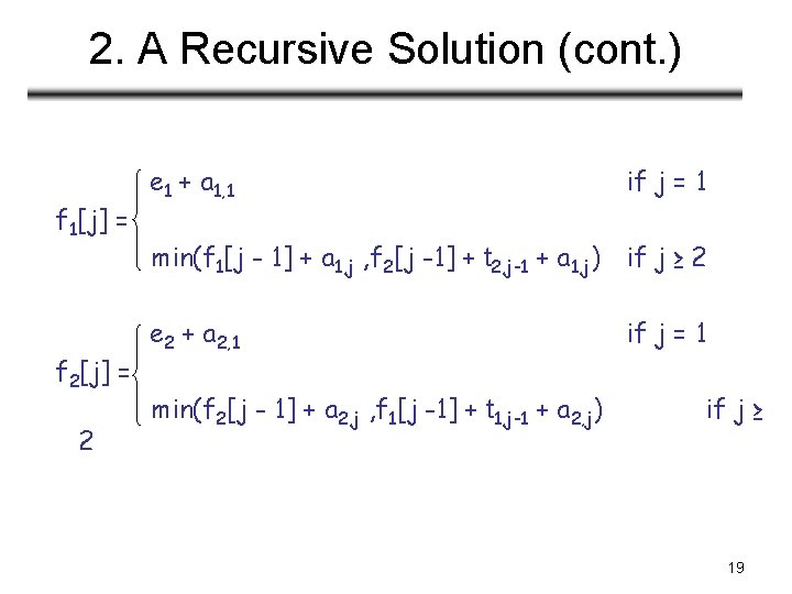
2. A Recursive Solution (cont. ) f 1[j] = f 2[j] = 2 e 1 + a 1, 1 if j = 1 min(f 1[j - 1] + a 1, j , f 2[j -1] + t 2, j-1 + a 1, j) if j ≥ 2 e 2 + a 2, 1 min(f 2[j - 1] + a 2, j , f 1[j -1] + t 1, j-1 + a 2, j) if j = 1 if j ≥ 19

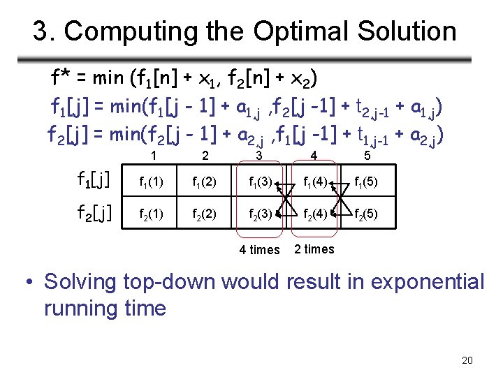
3. Computing the Optimal Solution f* = min (f 1[n] + x 1, f 2[n] + x 2) f 1[j] = min(f 1[j - 1] + a 1, j , f 2[j -1] + t 2, j-1 + a 1, j) f 2[j] = min(f 2[j - 1] + a 2, j , f 1[j -1] + t 1, j-1 + a 2, j) 1 2 3 4 5 f 1[j] f 1(1) f 1(2) f 1(3) f 1(4) f 1(5) f 2[j] f 2(1) f 2(2) f 2(3) f 2(4) f 2(5) 4 times 2 times • Solving top-down would result in exponential running time 20

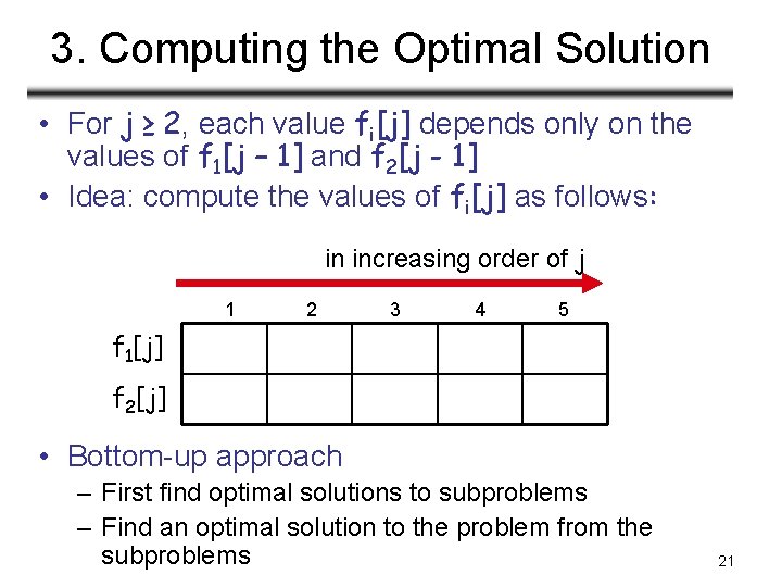
3. Computing the Optimal Solution • For j ≥ 2, each value fi[j] depends only on the values of f 1[j – 1] and f 2[j - 1] • Idea: compute the values of fi[j] as follows: in increasing order of j 1 2 3 4 5 f 1[j] f 2[j] • Bottom-up approach – First find optimal solutions to subproblems – Find an optimal solution to the problem from the subproblems 21

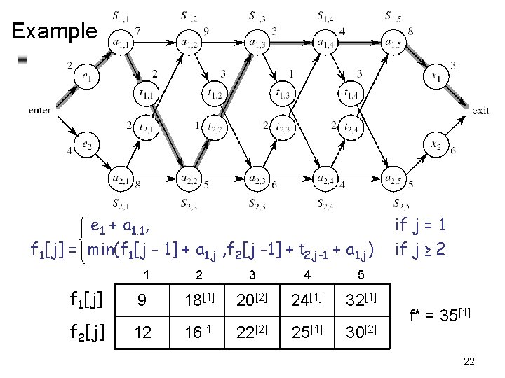
Example e 1 + a 1, 1, f 1[j] = min(f 1[j - 1] + a 1, j , f 2[j -1] + t 2, j-1 + a 1, j) 1 2 3 4 5 f 1[j] 9 18[1] 20[2] 24[1] 32[1] f 2[j] 12 16[1] 22[2] 25[1] 30[2] if j = 1 if j ≥ 2 f* = 35[1] 22

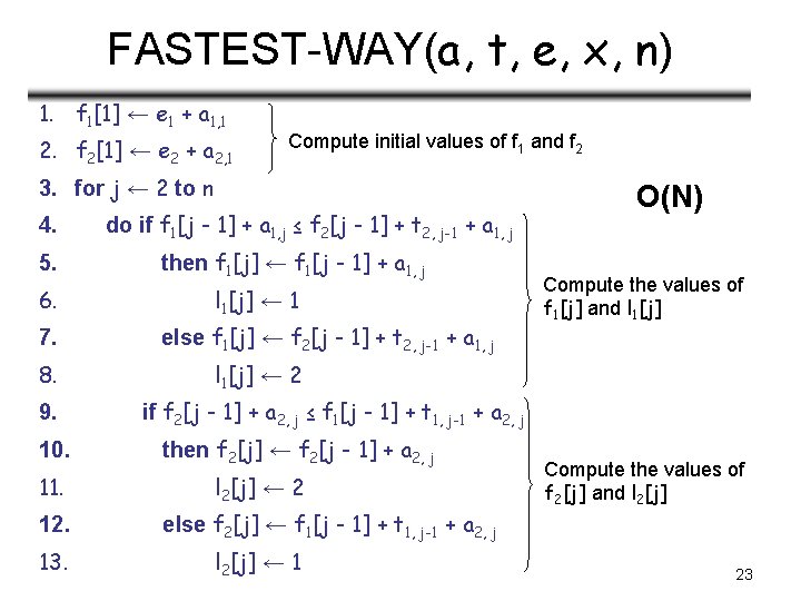
FASTEST-WAY(a, t, e, x, n) 1. f 1[1] ← e 1 + a 1, 1 2. f 2[1] ← e 2 + a 2, 1 Compute initial values of f 1 and f 2 3. for j ← 2 to n 4. 5. 6. 7. 8. 9. 10. 11. 12. 13. do if f 1[j - 1] + a 1, j ≤ f 2[j - 1] + t 2, j-1 + a 1, j then f 1[j] ← f 1[j - 1] + a 1, j l 1[j] ← 1 else f 1[j] ← f 2[j - 1] + t 2, j-1 + a 1, j O(N) Compute the values of f 1[j] and l 1[j] ← 2 if f 2[j - 1] + a 2, j ≤ f 1[j - 1] + t 1, j-1 + a 2, j then f 2[j] ← f 2[j - 1] + a 2, j l 2[j] ← 2 else f 2[j] ← f 1[j - 1] + t 1, j-1 + a 2, j l 2[j] ← 1 Compute the values of f 2[j] and l 2[j] 23

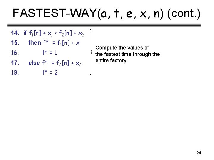
FASTEST-WAY(a, t, e, x, n) (cont. ) 14. if f 1[n] + x 1 ≤ f 2[n] + x 2 15. 16. 17. 18. then f* = f 1[n] + x 1 l* = 1 else f* = f 2[n] + x 2 Compute the values of the fastest time through the entire factory l* = 2 24

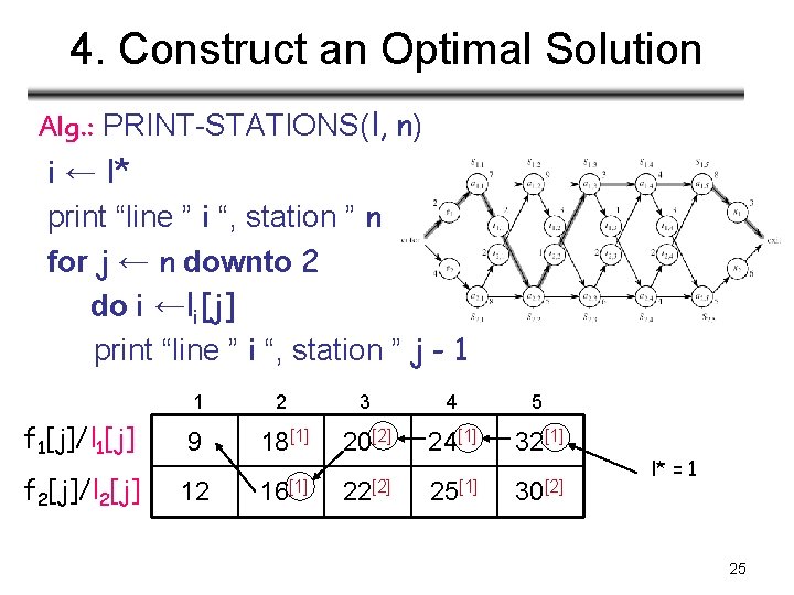
4. Construct an Optimal Solution Alg. : PRINT-STATIONS(l, n) i ← l* print “line ” i “, station ” n for j ← n downto 2 do i ←li[j] print “line ” i “, station ” j - 1 1 2 3 4 5 f 1[j]/l 1[j] 9 18[1] 20[2] 24[1] 32[1] f 2[j]/l 2[j] 12 16[1] 22[2] 25[1] 30[2] l* = 1 25

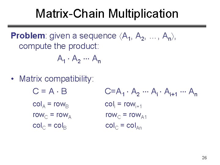
Matrix-Chain Multiplication Problem: given a sequence A 1, A 2, …, An , compute the product: A 1 A 2 An • Matrix compatibility: C=A B col. A = row. B row. C = row. A col. C = col. B C=A 1 A 2 Ai Ai+1 An coli = rowi+1 row. C = row. A 1 col. C = col. An 26

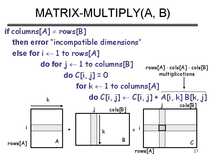
MATRIX-MULTIPLY(A, B) if columns[A] rows[B] then error “incompatible dimensions” else for i 1 to rows[A] do for j 1 to columns[B] rows[A] cols[B] multiplications do C[i, j] = 0 for k 1 to columns[A] do C[i, j] + A[i, k] B[k, j] k j i rows[A] * A j cols[B] = i k B C rows[A] 27

Matrix-Chain Multiplication • In what order should we multiply the matrices? A 1 A 2 An • Parenthesize the product to get the order in which matrices are multiplied • E. g. : A 1 A 2 A 3 = ((A 1 A 2) A 3) = (A 1 (A 2 A 3)) • Which one of these orderings should we choose? – The order in which we multiply the matrices has a significant impact on the cost of evaluating the product 28

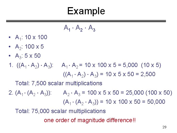
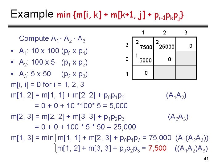
Example A 1 A 2 A 3 • A 1: 10 x 100 • A 2: 100 x 5 • A 3: 5 x 50 1. ((A 1 A 2) A 3): A 1 A 2 = 10 x 100 x 5 = 5, 000 (10 x 5) ((A 1 A 2) A 3) = 10 x 50 = 2, 500 Total: 7, 500 scalar multiplications 2. (A 1 (A 2 A 3)): A 2 A 3 = 100 x 50 = 25, 000 (100 x 50) (A 1 (A 2 A 3)) = 10 x 100 x 50 = 50, 000 Total: 75, 000 scalar multiplications one order of magnitude difference!! 29

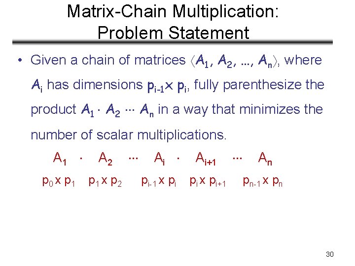
Matrix-Chain Multiplication: Problem Statement • Given a chain of matrices A 1, A 2, …, An , where Ai has dimensions pi-1 x pi, fully parenthesize the product A 1 A 2 An in a way that minimizes the number of scalar multiplications. A 1 p 0 x p 1 A 2 p 1 x p 2 Ai pi-1 x pi Ai+1 pi x pi+1 An pn-1 x pn 30

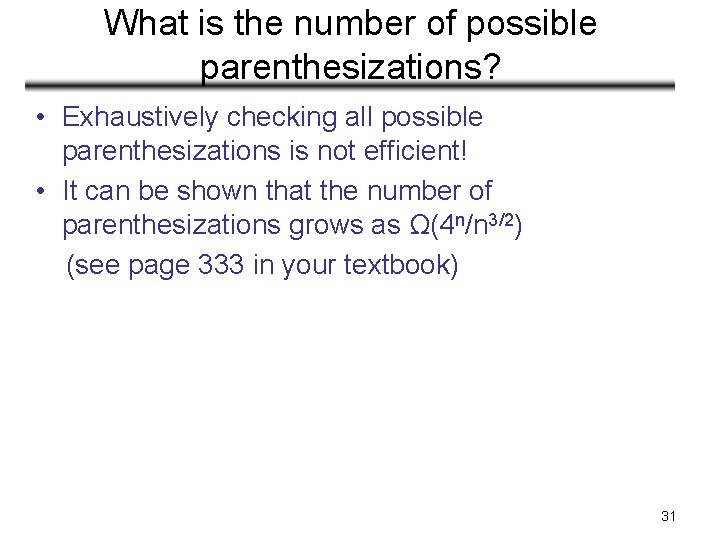
What is the number of possible parenthesizations? • Exhaustively checking all possible parenthesizations is not efficient! • It can be shown that the number of parenthesizations grows as Ω(4 n/n 3/2) (see page 333 in your textbook) 31

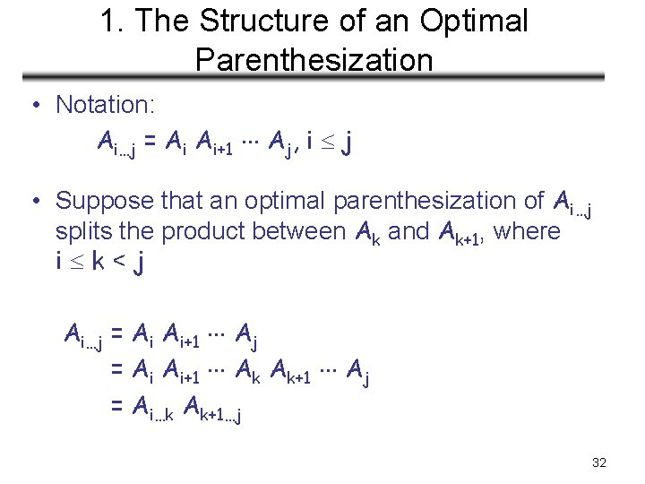
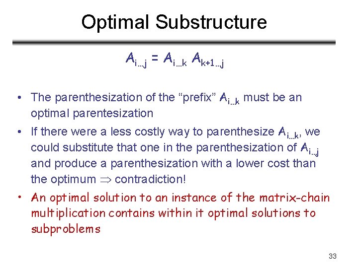
1. The Structure of an Optimal Parenthesization • Notation: Ai…j = Ai Ai+1 Aj, i j • Suppose that an optimal parenthesization of Ai…j splits the product between Ak and Ak+1, where i k<j Ai…j = Ai Ai+1 Ak Ak+1 Aj = Ai…k Ak+1…j 32

Optimal Substructure Ai…j = Ai…k Ak+1…j • The parenthesization of the “prefix” Ai…k must be an optimal parentesization • If there were a less costly way to parenthesize Ai…k, we could substitute that one in the parenthesization of Ai…j and produce a parenthesization with a lower cost than the optimum contradiction! • An optimal solution to an instance of the matrix-chain multiplication contains within it optimal solutions to subproblems 33

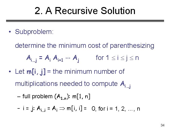
2. A Recursive Solution • Subproblem: determine the minimum cost of parenthesizing Ai…j = Ai Ai+1 Aj for 1 i j n • Let m[i, j] = the minimum number of multiplications needed to compute Ai…j – full problem (A 1. . n): m[1, n] – i = j: Ai…i = Ai m[i, i] = 0, for i = 1, 2, …, n 34

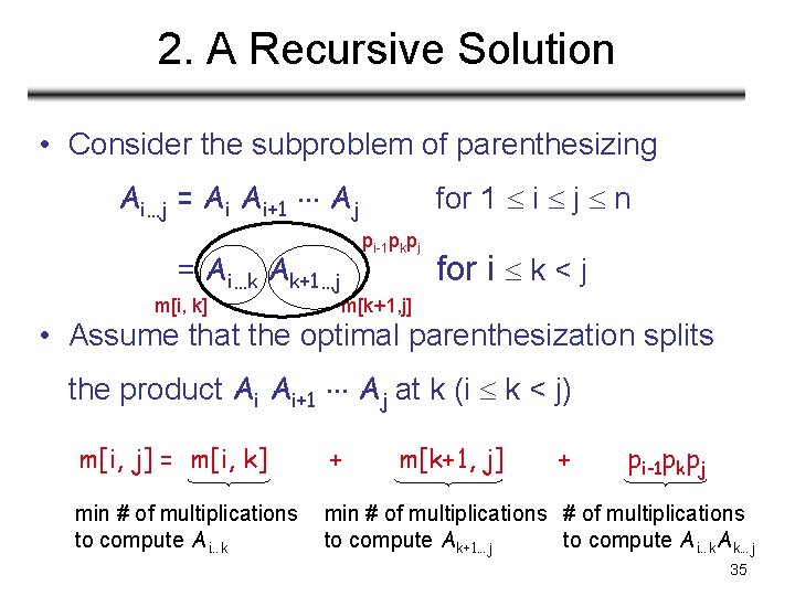
2. A Recursive Solution • Consider the subproblem of parenthesizing Ai…j = Ai Ai+1 Aj = Ai…k Ak+1…j m[i, k] for 1 i j n pi-1 pkpj for i k < j m[k+1, j] • Assume that the optimal parenthesization splits the product Ai Ai+1 Aj at k (i k < j) m[i, j] = m[i, k] + m[k+1, j] + p i-1 pkpj min # of multiplications to compute Ai…k min # of multiplications to compute Ak+1…j to compute Ai…k. Ak…j 35

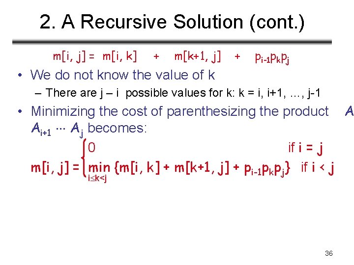
2. A Recursive Solution (cont. ) m[i, j] = m[i, k] + m[k+1, j] + pi-1 pkpj • We do not know the value of k – There are j – i possible values for k: k = i, i+1, …, j-1 • Minimizing the cost of parenthesizing the product A Ai+1 Aj becomes: 0 if i = j m[i, j] = min {m[i, k] + m[k+1, j] + pi-1 pkpj} if i < j i k<j 36

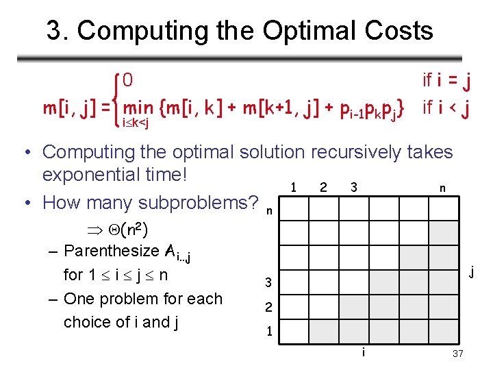
3. Computing the Optimal Costs 0 if i = j m[i, j] = min {m[i, k] + m[k+1, j] + pi-1 pkpj} if i < j i k<j • Computing the optimal solution recursively takes exponential time! 1 2 3 n • How many subproblems? n (n 2) – Parenthesize Ai…j for 1 i j n – One problem for each choice of i and j j 3 2 1 i 37

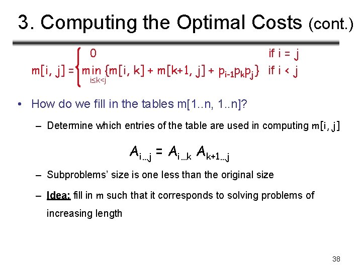
3. Computing the Optimal Costs (cont. ) 0 if i = j m[i, j] = min {m[i, k] + m[k+1, j] + pi-1 pkpj} if i < j i k<j • How do we fill in the tables m[1. . n, 1. . n]? – Determine which entries of the table are used in computing m[i, j] Ai…j = Ai…k Ak+1…j – Subproblems’ size is one less than the original size – Idea: fill in m such that it corresponds to solving problems of increasing length 38

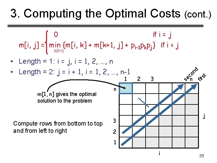
3. Computing the Optimal Costs (cont. ) 0 if i = j m[i, j] = min {m[i, k] + m[k+1, j] + pi-1 pkpj} if i < j i k<j • Length = 1: i = j, i = 1, 2, …, n • Length = 2: j = i + 1, i = 1, 2, …, n-1 1 m[1, n] gives the optimal solution to the problem Compute rows from bottom to top and from left to right 2 nd o t c s r e i s n f 3 n j 3 2 1 i 39

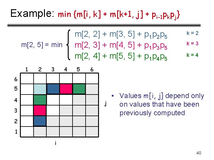
Example: min {m[i, k] + m[k+1, j] + pi-1 pkpj} m[2, 2] + m[3, 5] + p 1 p 2 p 5 m[2, 3] + m[4, 5] + p 1 p 3 p 5 m[2, 4] + m[5, 5] + p 1 p 4 p 5 m[2, 5] = min 1 2 3 4 5 k=2 k=3 k=4 6 6 5 4 j 3 • Values m[i, j] depend only on values that have been previously computed 2 1 i 40

Example min {m[i, k] + m[k+1, j] + pi-1 pkpj} Compute A 1 A 2 A 3 • A 1: 10 x 100 (p 0 x p 1) • A 2: 100 x 5 (p 1 x p 2) 1 3 2 2 1 7500 5000 2 2 3 25000 0 1 • A 3: 5 x 50 (p 2 x p 3) m[i, i] = 0 for i = 1, 2, 3 m[1, 2] = m[1, 1] + m[2, 2] + p 0 p 1 p 2 (A 1 A 2) = 0 + 10 *100* 5 = 5, 000 m[2, 3] = m[2, 2] + m[3, 3] + p 1 p 2 p 3 (A 2 A 3) = 0 + 100 * 50 = 25, 000 m[1, 3] = min m[1, 1] + m[2, 3] + p 0 p 1 p 3 = 75, 000 (A 1(A 2 A 3)) m[1, 2] + m[3, 3] + p 0 p 2 p 3 = 7, 500 ((A 1 A 2)A 3) 41

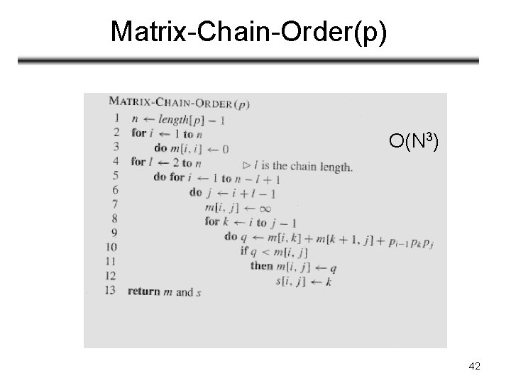
Matrix-Chain-Order(p) O(N 3) 42

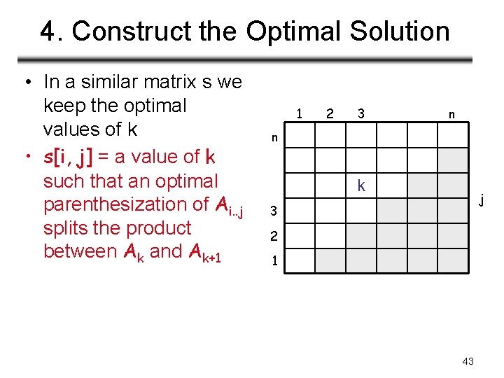
4. Construct the Optimal Solution • In a similar matrix s we keep the optimal values of k • s[i, j] = a value of k such that an optimal parenthesization of Ai. . j splits the product between Ak and Ak+1 1 2 3 n n k j 3 2 1 43

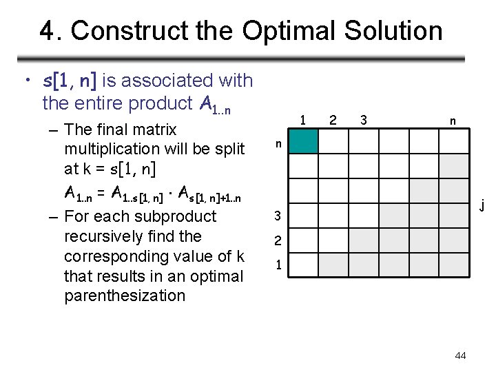
4. Construct the Optimal Solution • s[1, n] is associated with the entire product A 1. . n – The final matrix multiplication will be split at k = s[1, n] A 1. . n = A 1. . s[1, n] As[1, n]+1. . n – For each subproduct recursively find the corresponding value of k that results in an optimal parenthesization 1 2 3 n n j 3 2 1 44

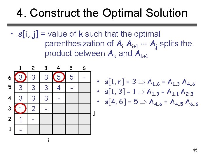
4. Construct the Optimal Solution • s[i, j] = value of k such that the optimal parenthesization of Ai Ai+1 Aj splits the product between Ak and Ak+1 6 5 4 3 2 1 1 2 3 4 5 6 3 3 3 1 3 3 3 2 3 3 3 - 5 4 - 5 - - 1 - - • s[1, n] = 3 A 1. . 6 = A 1. . 3 A 4. . 6 • s[1, 3] = 1 A 1. . 3 = A 1. . 1 A 2. . 3 • s[4, 6] = 5 A 4. . 6 = A 4. . 5 A 6. . 6 j i 45

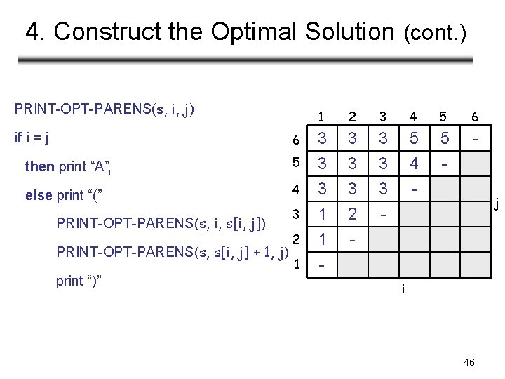
4. Construct the Optimal Solution (cont. ) PRINT-OPT-PARENS(s, i, j) if i = j 6 then print “A”i 5 else print “(” 4 PRINT-OPT-PARENS(s, i, s[i, j]) PRINT-OPT-PARENS(s, s[i, j] + 1, j) print “)” 3 2 1 1 2 3 4 5 6 3 3 3 1 3 3 3 2 3 3 3 - 5 4 - 5 - - 1 - - j i 46

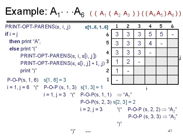
Example: A 1 A 6 ( ( A 1 ( A 2 A 3 ) ) ( ( A 4 A 5 ) A 6 ) ) PRINT-OPT-PARENS(s, i, j) s[1. . 6, 1. . 6] if i = j 6 then print “A”i 5 else print “(” 4 PRINT-OPT-PARENS(s, i, s[i, j]) PRINT-OPT-PARENS(s, s[i, j] + 1, j) 3 2 print “)” 1 2 3 4 5 6 3 3 3 1 3 3 3 2 3 3 3 - 5 4 - 5 - - 1 P-O-P(s, 1, 6) s[1, 6] = 3 i = 1, j = 6 “(“ P-O-P (s, 1, 3) s[1, 3] = 1 i i = 1, j = 3 “(“ P-O-P(s, 1, 1) “A 1” P-O-P(s, 2, 3) s[2, 3] = 2 i = 2, j = 3 “(“ P-O-P (s, 2, 2) “A 2” P-O-P (s, 3, 3) “A 3” “)” 47 … “)” j

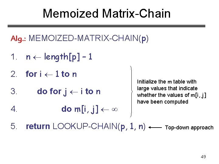
Memoization • Top-down approach with the efficiency of typical dynamic programming approach • Maintaining an entry in a table for the solution to each subproblem – memoize the inefficient recursive algorithm • When a subproblem is first encountered its solution is computed and stored in that table • Subsequent “calls” to the subproblem simply look up that value 48

Memoized Matrix-Chain Alg. : MEMOIZED-MATRIX-CHAIN(p) 1. n length[p] – 1 2. for i 1 to n 3. 4. do for j i to n do m[i, j] Initialize the m table with large values that indicate whether the values of m[i, j] have been computed 5. return LOOKUP-CHAIN(p, 1, n) Top-down approach 49

Memoized Matrix-Chain Alg. : LOOKUP-CHAIN(p, i, j) 1. 2. 3. if m[i, j] < then return m[i, j] if i = j 4. then m[i, j] 0 5. else for k i to j – 1 6. Running time is O(n 3) do q LOOKUP-CHAIN(p, i, k) + LOOKUP-CHAIN(p, k+1, j) + pi-1 pkpj 7. 8. 9. return m[i, j] if q < m[i, j] then m[i, j] q 50

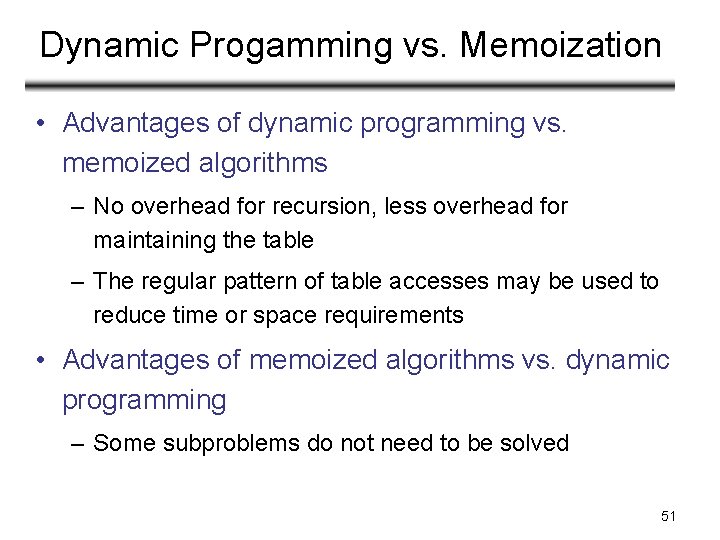
Dynamic Progamming vs. Memoization • Advantages of dynamic programming vs. memoized algorithms – No overhead for recursion, less overhead for maintaining the table – The regular pattern of table accesses may be used to reduce time or space requirements • Advantages of memoized algorithms vs. dynamic programming – Some subproblems do not need to be solved 51

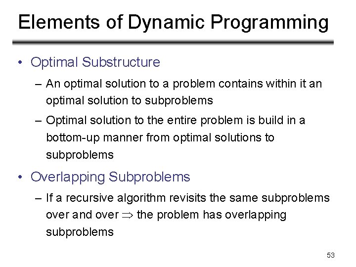
Elements of Dynamic Programming • Optimal Substructure – An optimal solution to a problem contains within it an optimal solution to subproblems – Optimal solution to the entire problem is build in a bottom-up manner from optimal solutions to subproblems • Overlapping Subproblems – If a recursive algorithm revisits the same subproblems over and over the problem has overlapping subproblems 53

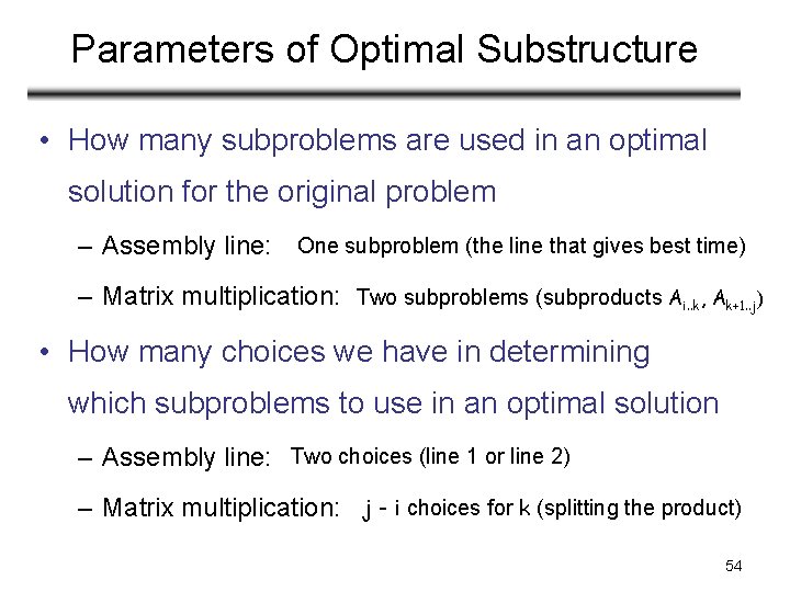
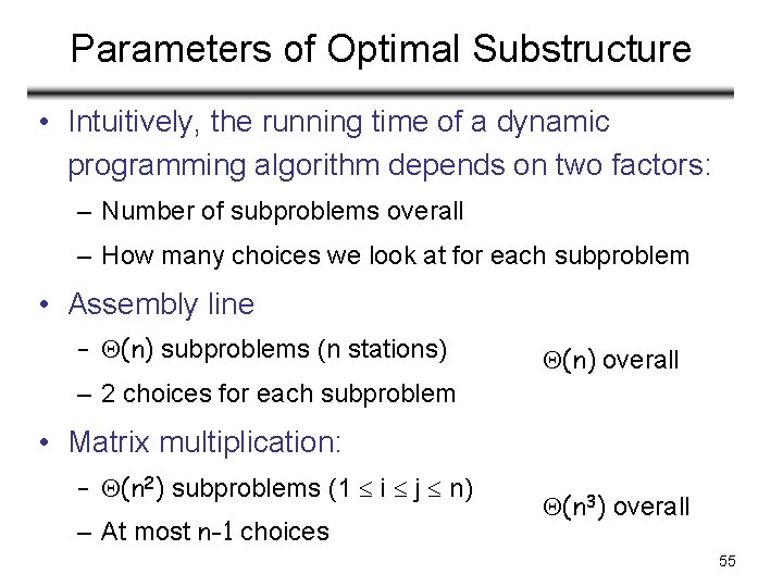
Parameters of Optimal Substructure • How many subproblems are used in an optimal solution for the original problem – Assembly line: One subproblem (the line that gives best time) – Matrix multiplication: Two subproblems (subproducts Ai. . k, Ak+1. . j) • How many choices we have in determining which subproblems to use in an optimal solution – Assembly line: Two choices (line 1 or line 2) – Matrix multiplication: j - i choices for k (splitting the product) 54

Parameters of Optimal Substructure • Intuitively, the running time of a dynamic programming algorithm depends on two factors: – Number of subproblems overall – How many choices we look at for each subproblem • Assembly line – (n) subproblems (n stations) (n) overall – 2 choices for each subproblem • Matrix multiplication: – (n 2) subproblems (1 i j n) – At most n-1 choices (n 3) overall 55

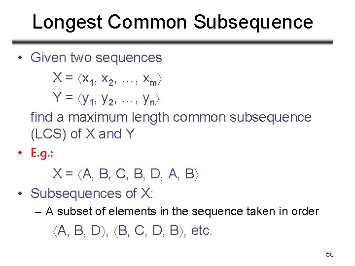
Longest Common Subsequence • Given two sequences X = x 1, x 2, …, xm Y = y 1, y 2, …, yn find a maximum length common subsequence (LCS) of X and Y • E. g. : X = A, B, C, B, D, A, B • Subsequences of X: – A subset of elements in the sequence taken in order A, B, D , B, C, D, B , etc. 56

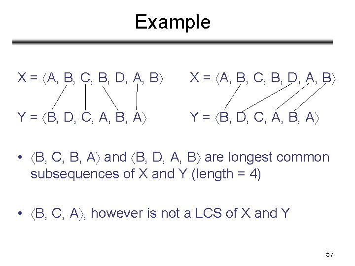
Example X = A, B, C, B, D, A, B Y = B, D, C, A, B, A • B, C, B, A and B, D, A, B are longest common subsequences of X and Y (length = 4) • B, C, A , however is not a LCS of X and Y 57

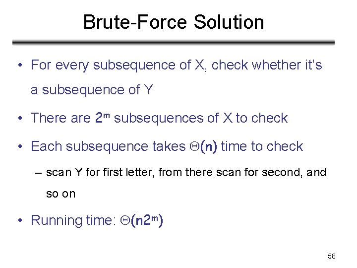
Brute-Force Solution • For every subsequence of X, check whether it’s a subsequence of Y • There are 2 m subsequences of X to check • Each subsequence takes (n) time to check – scan Y for first letter, from there scan for second, and so on • Running time: (n 2 m) 58

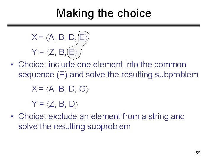
Making the choice X = A, B, D, E Y = Z, B, E • Choice: include one element into the common sequence (E) and solve the resulting subproblem X = A, B, D, G Y = Z, B, D • Choice: exclude an element from a string and solve the resulting subproblem 59

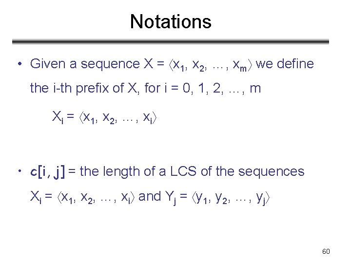
Notations • Given a sequence X = x 1, x 2, …, xm we define the i-th prefix of X, for i = 0, 1, 2, …, m Xi = x 1, x 2, …, xi • c[i, j] = the length of a LCS of the sequences Xi = x 1, x 2, …, xi and Yj = y 1, y 2, …, yj 60

A Recursive Solution Case 1: xi = yj e. g. : Xi = A, B, D, E Yj = Z, B, E c[i, j] = c[i - 1, j - 1] + 1 – Append xi = yj to the LCS of Xi-1 and Yj-1 – Must find a LCS of Xi-1 and Yj-1 optimal solution to a problem includes optimal solutions to subproblems 61

A Recursive Solution Case 2: xi yj e. g. : Xi = A, B, D, G Yj = Z, B, D c[i, j] = max { c[i - 1, j], c[i, j-1] } – Must solve two problems • find a LCS of Xi-1 and Yj: Xi-1 = A, B, D and Yj = Z, B, D • find a LCS of Xi and Yj-1: Xi = A, B, D, G and Yj = Z, B • Optimal solution to a problem includes optimal solutions to subproblems 62

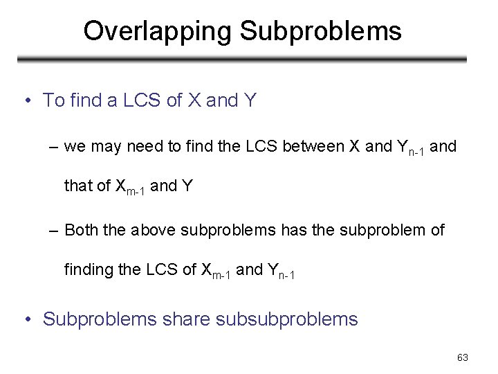
Overlapping Subproblems • To find a LCS of X and Y – we may need to find the LCS between X and Yn-1 and that of Xm-1 and Y – Both the above subproblems has the subproblem of finding the LCS of Xm-1 and Yn-1 • Subproblems share subsubproblems 63

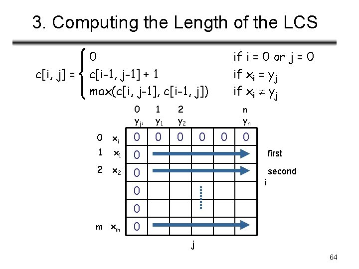
3. Computing the Length of the LCS c[i, j] = 0 c[i-1, j-1] + 1 max(c[i, j-1], c[i-1, j]) 0 xi 1 x 1 2 x 2 m xm 0 yj: 1 y 1 2 y 2 0 0 0 if i = 0 or j = 0 if xi = yj if xi yj n yn 0 0 0 first i second 0 0 j 64

Additional Information 0 if i, j = 0 c[i, j] = c[i-1, j-1] + 1 if xi = yj max(c[i, j-1], c[i-1, j]) if xi yj b & c: 0 yj: 1 A 2 C 3 D 0 0 xi 1 A 2 B 3 C 0 0 m D 0 0 c[i-1, j] c[i, j-1] j n F 0 0 i A matrix b[i, j]: • For a subproblem [i, j] it tells us what choice was made to obtain the optimal value • If xi = yj b[i, j] = “ ” • Else, if c[i - 1, j] ≥ c[i, j-1] b[i, j] = “ ” else b[i, j] = “ ” 65

LCS-LENGTH(X, Y, m, n) 1. for i ← 1 to m 2. do c[i, 0] ← 0 The length of the LCS if one of the sequences 3. for j ← 0 to n is empty is zero 4. do c[0, j] ← 0 5. for i ← 1 to m 6. do for j ← 1 to n 7. do if xi = yj 8. then c[i, j] ← c[i - 1, j - 1] + 1 Case 1: xi = yj 9. b[i, j ] ← “ ” 10. else if c[i - 1, j] ≥ c[i, j - 1] 11. then c[i, j] ← c[i - 1, j] 12. b[i, j] ← “↑” Case 2: xi yj 13. else c[i, j] ← c[i, j - 1] 14. b[i, j] ← “←” 15. return c and b Running time: (mn) 66

Example 0 if i = 0 or j = 0 if xi = yj max(c[i, j-1], c[i-1, j]) if xi yj X = A, B, C, B, D, A c[i, j] = c[i-1, j-1] + 1 Y = B, D, C, A, B, A If xi = yj b[i, j] = “ ” Else if c[i - 1, j] ≥ c[i, j-1] b[i, j] = “ ” else b[i, j] = “ ” 0 yj 1 B 2 D 3 C 4 A 5 B 6 A 0 0 0 1 1 1 1 0 xi 0 0 1 A 0 0 2 B 0 3 C 0 1 1 4 B 0 5 D 0 6 A 0 1 1 1 7 B 0 1 2 2 2 3 3 2 2 3 3 3 4 4 4 67

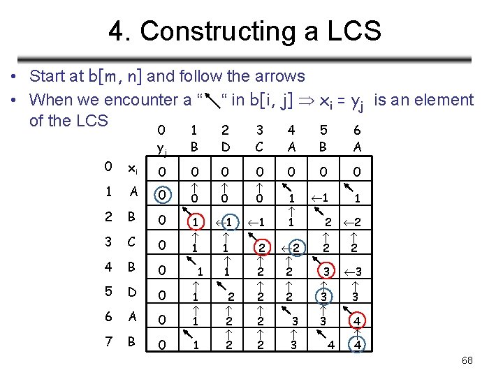
4. Constructing a LCS • Start at b[m, n] and follow the arrows • When we encounter a “ “ in b[i, j] xi = yj is an element of the LCS 0 yj 1 B 2 D 3 C 4 A 5 B 6 A 0 0 0 1 1 1 1 0 xi 0 0 1 A 0 0 2 B 0 3 C 0 1 1 4 B 0 5 D 0 6 A 0 1 1 1 7 B 0 1 2 2 2 3 3 2 2 3 3 3 4 4 4 68

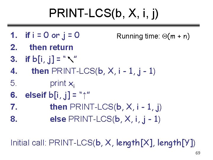
PRINT-LCS(b, X, i, j) 1. if i = 0 or j = 0 Running time: (m + n) 2. then return 3. if b[i, j] = “ ” 4. then PRINT-LCS(b, X, i - 1, j - 1) 5. print xi 6. elseif b[i, j] = “↑” 7. then PRINT-LCS(b, X, i - 1, j) 8. else PRINT-LCS(b, X, i, j - 1) Initial call: PRINT-LCS(b, X, length[X], length[Y]) 69

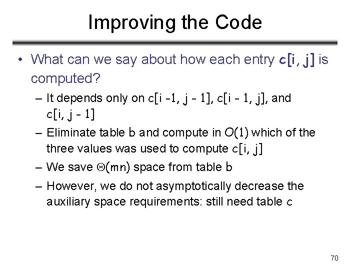
Improving the Code • What can we say about how each entry c[i, j] is computed? – It depends only on c[i -1, j - 1], c[i - 1, j], and c[i, j - 1] – Eliminate table b and compute in O(1) which of the three values was used to compute c[i, j] – We save (mn) space from table b – However, we do not asymptotically decrease the auxiliary space requirements: still need table c 70

Improving the Code • If we only need the length of the LCS – LCS-LENGTH works only on two rows of c at a time • The row being computed and the previous row – We can reduce the asymptotic space requirements by storing only these two rows 71