Analysis of Algorithms CMPE 371 Lecture GRAPHS Graphs

Analysis of Algorithms CMPE 371 Lecture GRAPHS

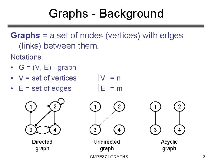
Graphs - Background Graphs = a set of nodes (vertices) with edges (links) between them. Notations: • G = (V, E) - graph • V = set of vertices • E = set of edges V = n E = m 1 2 1 2 3 4 3 4 Directed graph Undirected graph CMPE 371 GRAPHS Acyclic graph 2

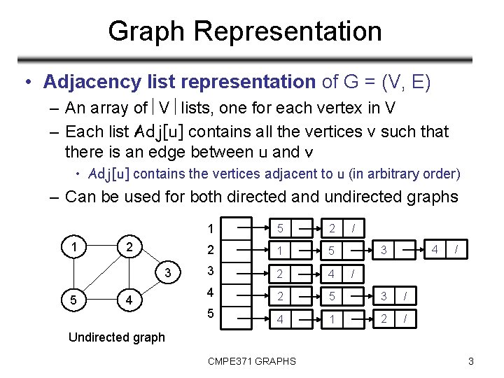
Graph Representation • Adjacency list representation of G = (V, E) – An array of V lists, one for each vertex in V – Each list Adj[u] contains all the vertices v such that there is an edge between u and v • Adj[u] contains the vertices adjacent to u (in arbitrary order) – Can be used for both directed and undirected graphs 1 2 3 5 4 1 5 2 2 1 5 3 2 4 4 2 5 3 / 5 4 1 2 / / 4 3 / / Undirected graph CMPE 371 GRAPHS 3

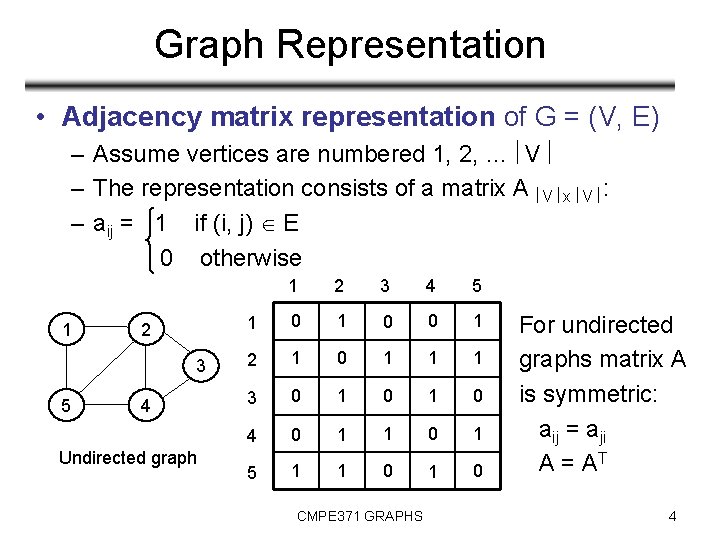
Graph Representation • Adjacency matrix representation of G = (V, E) – Assume vertices are numbered 1, 2, … V – The representation consists of a matrix A V x V : – aij = 1 if (i, j) E 0 otherwise 1 2 3 5 4 Undirected graph 1 2 3 4 5 1 0 0 1 2 1 0 1 1 1 3 0 1 0 4 0 1 1 0 1 5 1 1 0 CMPE 371 GRAPHS For undirected graphs matrix A is symmetric: aij = aji A = AT 4

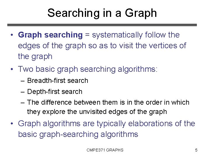
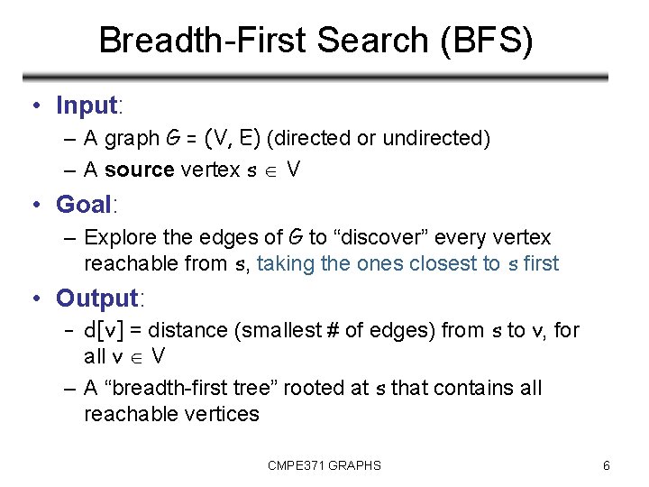
Searching in a Graph • Graph searching = systematically follow the edges of the graph so as to visit the vertices of the graph • Two basic graph searching algorithms: – Breadth-first search – Depth-first search – The difference between them is in the order in which they explore the unvisited edges of the graph • Graph algorithms are typically elaborations of the basic graph-searching algorithms CMPE 371 GRAPHS 5

Breadth-First Search (BFS) • Input: – A graph G = (V, E) (directed or undirected) – A source vertex s V • Goal: – Explore the edges of G to “discover” every vertex reachable from s, taking the ones closest to s first • Output: – d[v] = distance (smallest # of edges) from s to v, for all v V – A “breadth-first tree” rooted at s that contains all reachable vertices CMPE 371 GRAPHS 6

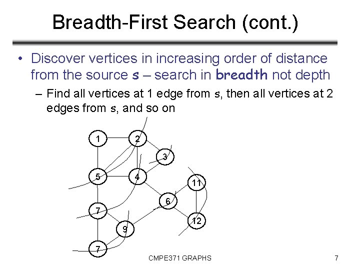
Breadth-First Search (cont. ) • Discover vertices in increasing order of distance from the source s – search in breadth not depth – Find all vertices at 1 edge from s, then all vertices at 2 edges from s, and so on 2 1 3 5 4 6 7 9 7 11 12 CMPE 371 GRAPHS 7

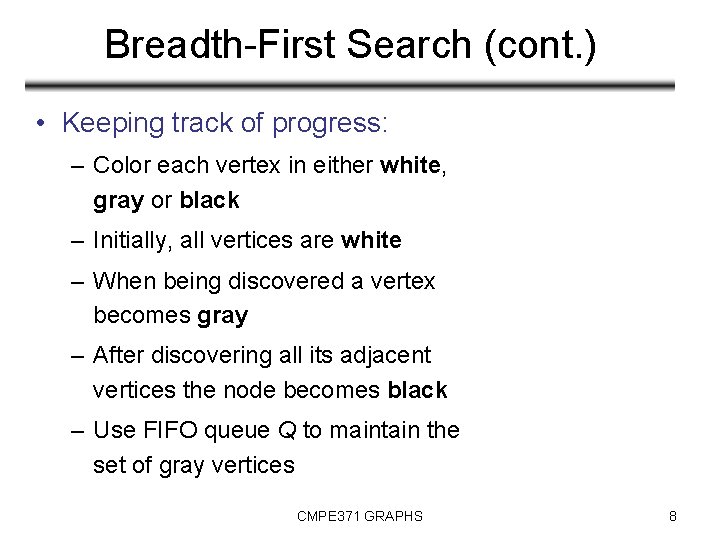
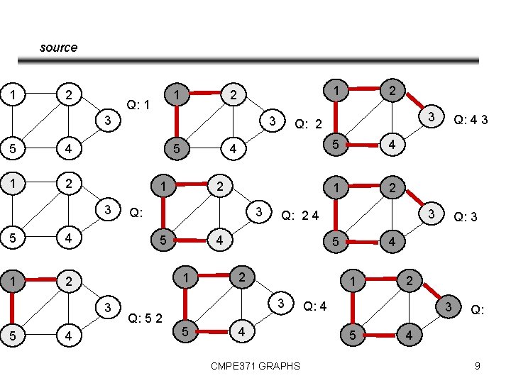
Breadth-First Search (cont. ) • Keeping track of progress: – Color each vertex in either white, gray or black – Initially, all vertices are white – When being discovered a vertex becomes gray – After discovering all its adjacent vertices the node becomes black – Use FIFO queue Q to maintain the set of gray vertices CMPE 371 GRAPHS 8

source 1 2 Q: 1 3 5 4 1 2 5 4 2 3 Q: 5 5 4 1 2 5 2 4 CMPE 371 GRAPHS 3 Q: 4 3 3 Q: 3 4 1 3 Q: 5 2 5 Q: 2 4 4 1 3 Q: 2 4 1 3 5 2 1 2 Q: 4 3 5 Q: 4 9

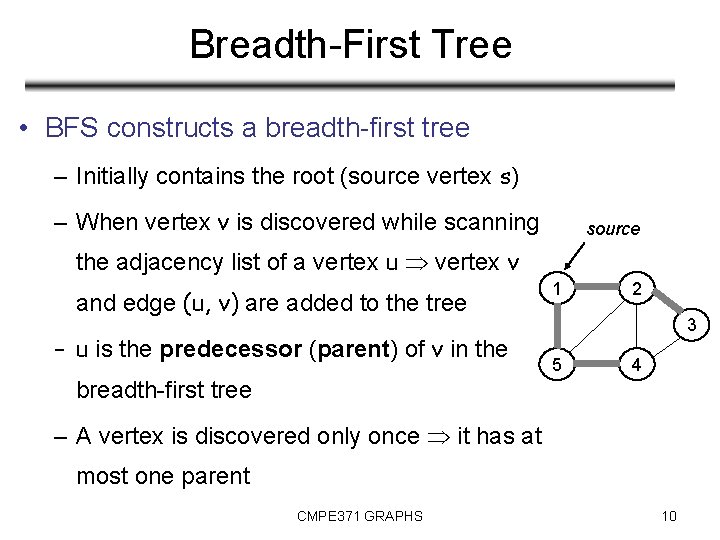
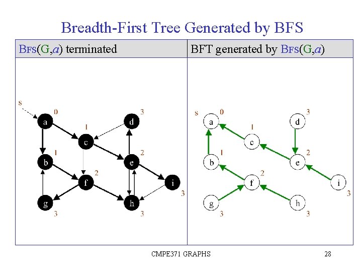
Breadth-First Tree • BFS constructs a breadth-first tree – Initially contains the root (source vertex s) – When vertex v is discovered while scanning source the adjacency list of a vertex u vertex v and edge (u, v) are added to the tree – u is the predecessor (parent) of v in the 1 2 3 5 4 breadth-first tree – A vertex is discovered only once it has at most one parent CMPE 371 GRAPHS 10

BFS Additional Data Structures • G = (V, E) represented using adjacency lists • color[u] – the color of the vertex for all u V • [u] – predecessor of u – If u = s (root) or node u has not yet been 1 source d=1 =1 2 3 discovered [u] = NIL • d[u] – the distance from the source s to vertex u 5 4 d=1 =1 d=2 =5 d=2 =2 • Use a FIFO queue Q to maintain the set of gray vertices CMPE 371 GRAPHS 11

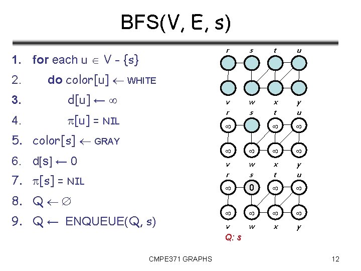
BFS(V, E, s) 1. for each u V - {s} 2. r s t u v r w s x t y u do color[u] WHITE 3. d[u] ← 4. [u] = NIL 5. color[s] GRAY 6. d[s] ← 0 7. [s] = NIL 8. Q 9. Q ← ENQUEUE(Q, s) v r w s x t y u 0 v w x y Q: s CMPE 371 GRAPHS 12

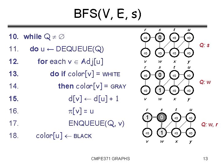
BFS(V, E, s) 10. while Q 11. do u ← DEQUEUE(Q) 12. for each v Adj[u] 13. do if color[v] = WHITE 14. then color[v] = GRAY 15. d[v] ← d[u] + 1 16. [v] = u 17. ENQUEUE(Q, v) 18. color[u] BLACK CMPE 371 GRAPHS r s t u 0 Q: s v r w s x t y u 0 Q: w 1 v w x y r s t u 1 0 Q: w, r 1 v w x y 13

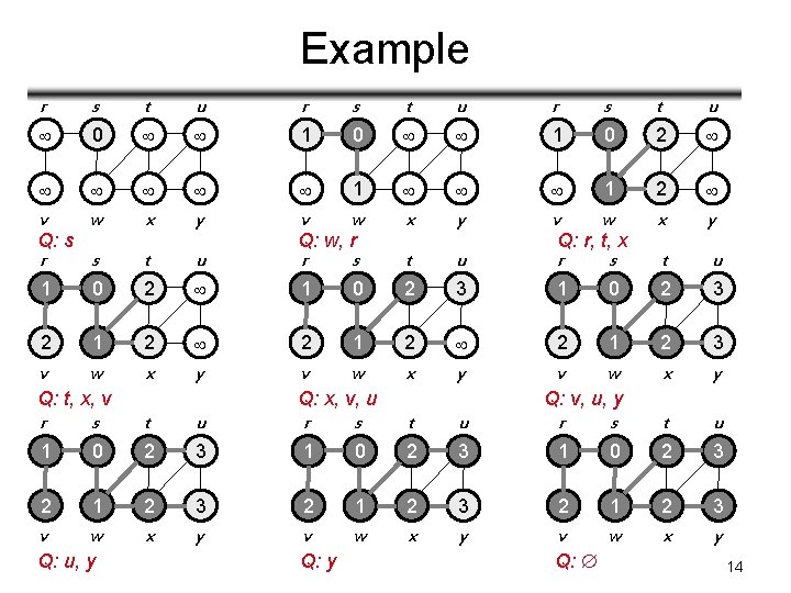
Example r s t u 0 1 0 2 1 1 2 v w x y r s t u 1 0 2 3 2 1 2 3 v w x y Q: s Q: t, x, v Q: w, r Q: x, v, u Q: r, t, x Q: v, u, y r s t u 1 0 2 3 2 1 2 3 v w x y Q: u, y Q: CMPE 371 y GRAPHS Q: 14

Analysis of BFS 1. for each u V - {s} 2. do color[u] WHITE 3. d[u] ← 4. [u] = NIL O(V) 5. color[s] GRAY 6. d[s] ← 0 7. [s] = NIL (1) 8. Q 9. Q ← ENQUEUE(Q, s) CMPE 371 GRAPHS 15

Analysis of BFS 10. while Q 11. do u ← DEQUEUE(Q) 12. for each v Adj[u] 13. do if color[v] = WHITE 14. then color[v] = GRAY 15. d[v] ← d[u] + 1 16. [v] = u 17. ENQUEUE(Q, v) 18. (1) Scan Adj[u] for all vertices in the graph • Each vertex is scanned only once, when the vertex is dequeued • Sum of lengths of all adjacency lists = (E) • Scanning operations: O(E) (1) color[u] BLACK • Total running time for BFS = O(V + E) CMPE 371 GRAPHS 16

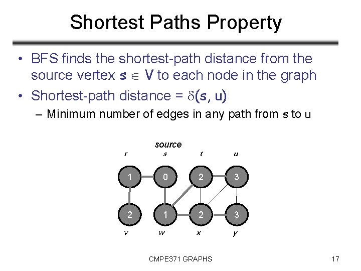
Shortest Paths Property • BFS finds the shortest-path distance from the source vertex s V to each node in the graph • Shortest-path distance = (s, u) – Minimum number of edges in any path from s to u source r v s t u 1 0 2 3 2 1 2 3 x y w CMPE 371 GRAPHS 17

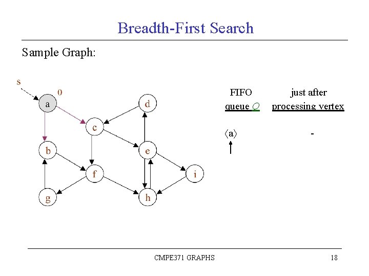
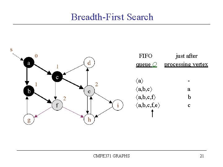
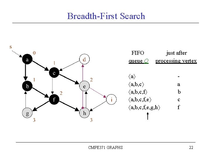
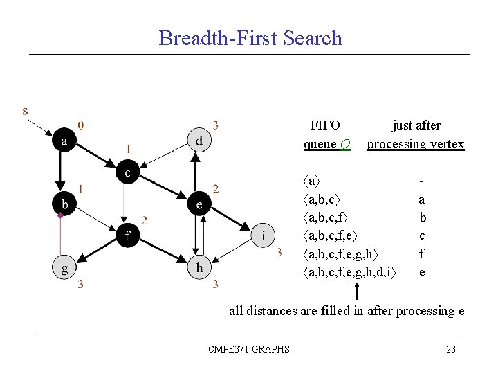
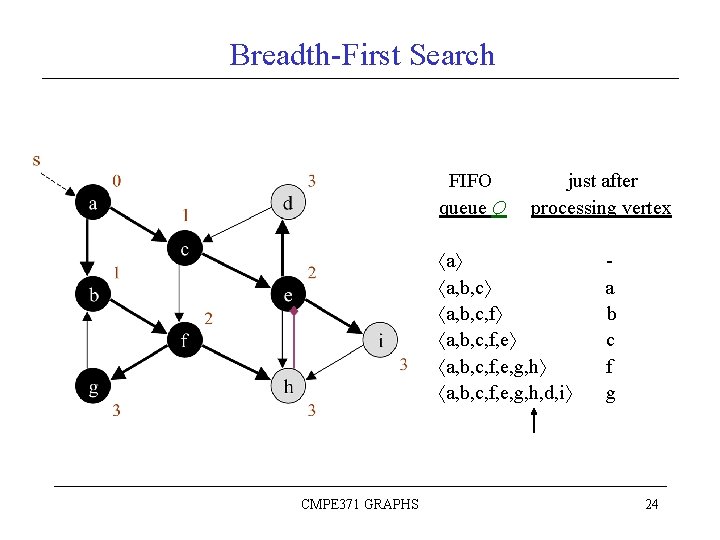
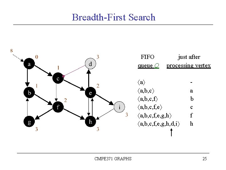
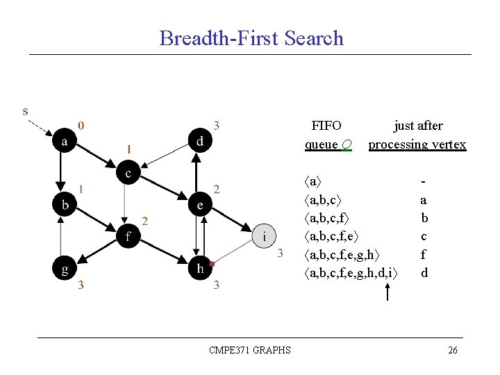
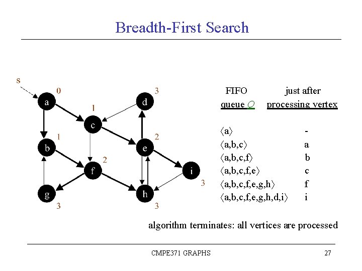
Breadth-First Search Sample Graph: FIFO queue Q a CMPE 371 GRAPHS just after processing vertex - 18

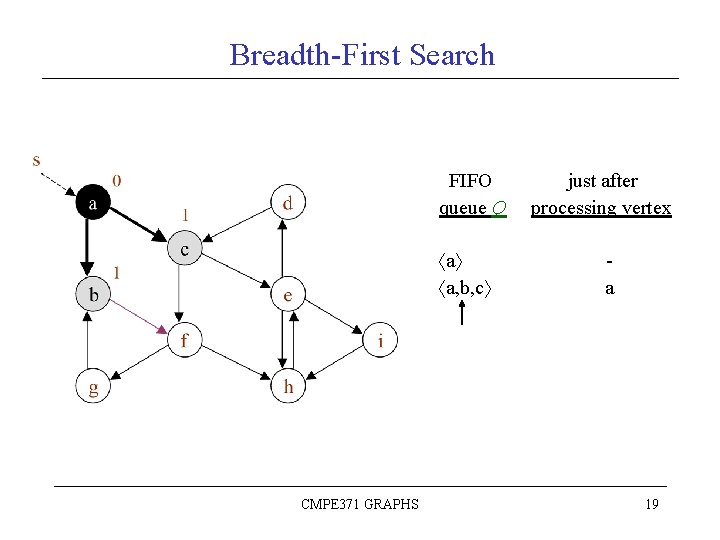
Breadth-First Search FIFO queue Q a a, b, c CMPE 371 GRAPHS just after processing vertex a 19

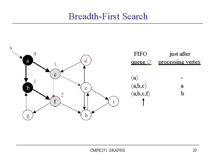
Breadth-First Search FIFO queue Q a a, b, c, f CMPE 371 GRAPHS just after processing vertex a b 20

Breadth-First Search FIFO queue Q a a, b, c, f, e CMPE 371 GRAPHS just after processing vertex a b c 21

Breadth-First Search FIFO queue Q just after processing vertex a a, b, c, f, e, g, h CMPE 371 GRAPHS a b c f 22

Breadth-First Search FIFO queue Q just after processing vertex a a, b, c, f, e, g, h a, b, c, f, e, g, h, d, i a b c f e all distances are filled in after processing e CMPE 371 GRAPHS 23

Breadth-First Search FIFO queue Q just after processing vertex a a, b, c, f, e, g, h a, b, c, f, e, g, h, d, i CMPE 371 GRAPHS a b c f g 24

Breadth-First Search FIFO queue Q just after processing vertex a a, b, c, f, e, g, h a, b, c, f, e, g, h, d, i CMPE 371 GRAPHS a b c f h 25

Breadth-First Search FIFO queue Q just after processing vertex a a, b, c, f, e, g, h a, b, c, f, e, g, h, d, i CMPE 371 GRAPHS a b c f d 26

Breadth-First Search FIFO queue Q just after processing vertex a a, b, c, f, e, g, h a, b, c, f, e, g, h, d, i a b c f i algorithm terminates: all vertices are processed CMPE 371 GRAPHS 27

Breadth-First Tree Generated by BFS(G, a) terminated BFT generated by BFS(G, a) CMPE 371 GRAPHS 28

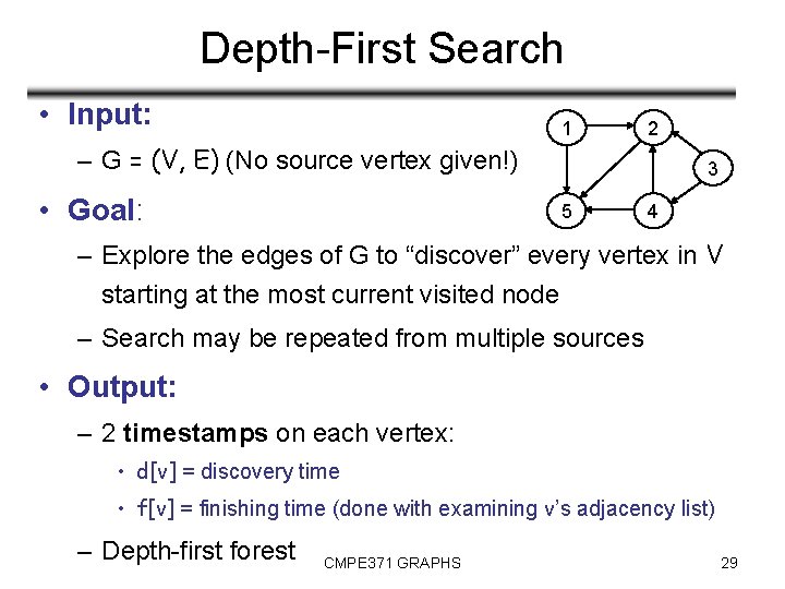
Depth-First Search • Input: 1 2 – G = (V, E) (No source vertex given!) • Goal: 3 5 4 – Explore the edges of G to “discover” every vertex in V starting at the most current visited node – Search may be repeated from multiple sources • Output: – 2 timestamps on each vertex: • d[v] = discovery time • f[v] = finishing time (done with examining v’s adjacency list) – Depth-first forest CMPE 371 GRAPHS 29

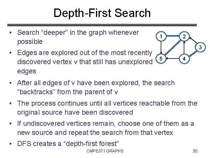
Depth-First Search • Search “deeper” in the graph whenever possible • Edges are explored out of the most recently discovered vertex v that still has unexplored edges 1 2 3 5 4 • After all edges of v have been explored, the search “backtracks” from the parent of v • The process continues until all vertices reachable from the original source have been discovered • If undiscovered vertices remain, choose one of them as a new source and repeat the search from that vertex • DFS creates a “depth-first forest” CMPE 371 GRAPHS 30

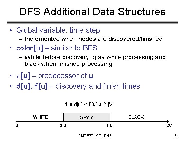
DFS Additional Data Structures • Global variable: time-step – Incremented when nodes are discovered/finished • color[u] – similar to BFS – White before discovery, gray while processing and black when finished processing • [u] – predecessor of u • d[u], f[u] – discovery and finish times 1 ≤ d[u] < f [u] ≤ 2 |V| WHITE 0 BLACK GRAY d[u] f[u] CMPE 371 GRAPHS 2 V 31

DFS(V, E) 1. for each u V 2. do color[u] ← WHITE 3. [u] ← NIL 4. time ← 0 5. for each u V 6. do if color[u] = WHITE 7. then DFS-VISIT(u) • u v w x y z Every time DFS-VISIT(u) is called, u becomes the root of a new tree in the depth-first forest CMPE 371 GRAPHS 32

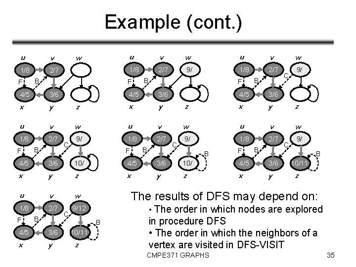
DFS-VISIT(u) 1. color[u] ← GRAY 2. time ← time+1 3. d[u] ← time 4. for each v Adj[u] 5. do if color[v] = WHITE 6. then [v] ← u 7. DFS-VISIT(v) 8. color[u] ← BLACK 9. time ← time + 1 10. f[u] ← time CMPE 371 GRAPHS u v w x y z time = 1 u v w x u y z v w 1/ 2/ x y 1/ z 33

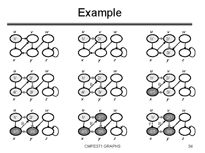
Example u v w 1/ u v 1/ 2/ w 3/ x y z u v w 1/ 2/ B 4/ 3/ x y u v 1/ 2/ B 4/ 3/ z x y w u v 1/ 2/7 B 4/5 3/ z x y z w u v w 1/ 2/7 B 4/5 3/6 x y z F 4/5 3/6 x y z CMPE 371 GRAPHS B 4/5 3/6 x y z 34

Example (cont. ) u v 1/8 2/7 F B u v w u v 1/8 2/7 9/ 1/8 2/7 F 4/5 3/6 x y u v 1/8 2/7 F w B C B F 4/5 3/6 z x y w u v 9/ 1/8 2/7 B F C B z x y z w u v w 9/ 1/8 2/7 B F B 4/5 3/6 10/ 4/5 3/6 x y z x y u v w 1/8 2/7 3/6 x y z 10/11 z • The order in which nodes are explored 9/12 10/11 9/ The results of DFS may depend on: B 4/5 C B 10/ B 9/ 3/6 F C 4/5 C w in procedure DFS • The order in which the neighbors of a vertex are visited in DFS-VISIT CMPE 371 GRAPHS 35

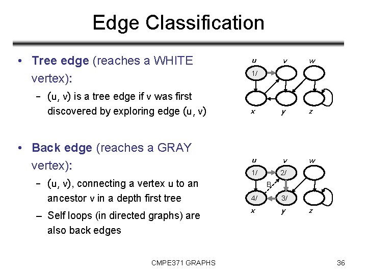
Edge Classification • Tree edge (reaches a WHITE vertex): – (u, v) is a tree edge if v was first discovered by exploring edge (u, v) • Back edge (reaches a GRAY vertex): – (u, v), connecting a vertex u to an ancestor v in a depth first tree – Self loops (in directed graphs) are also back edges CMPE 371 GRAPHS u v w x y z u v w 1/ 2/ 1/ B 4/ 3/ x y z 36

Edge Classification • Forward edge (reaches a BLACK vertex & d[u] < d[v]): – Non-tree edges (u, v) that connect a vertex u to a descendant v in a depth first tree • Cross edge (reaches a BLACK vertex & d[u] > d[v]): – Can go between vertices in same depth-first tree (as long as there is no ancestor / descendant relation) or between different depth-first trees CMPE 371 GRAPHS u v 1/ 2/7 F w B 4/5 3/6 x y z u v w 1/8 2/7 F B 4/5 3/6 x y C 9/ z 37

Analysis of DFS(V, E) 1. for each u V 2. do color[u] ← WHITE (V) 3. [u] ← NIL 4. time ← 0 5. for each u V (V) – exclusive 6. do if color[u] = WHITE of time for 7. then DFS-VISIT(u) DFS-VISIT CMPE 371 GRAPHS 38

Analysis of DFS-VISIT(u) 1. color[u] ← GRAY DFS-VISIT is called exactly once for each vertex 2. time ← time+1 3. d[u] ← time 4. for each v Adj[u] 5. do if color[v] = WHITE Each loop takes |Adj[v]| 6. then [v] ← u 7. DFS-VISIT(v) 8. color[u] ← BLACK 9. time ← time + 1 Total: Σv V |Adj[v]| + (V) = (V + E) 10. f[u] ← time (E) CMPE 371 GRAPHS 39

Properties of DFS • u = [v] DFS-VISIT(v) was called during a search of u’s adjacency list • Vertex v is a descendant of vertex u u v 1/ 2/ w 3/ x y z in the depth first forest v is discovered during the time in which u is gray CMPE 371 GRAPHS 40

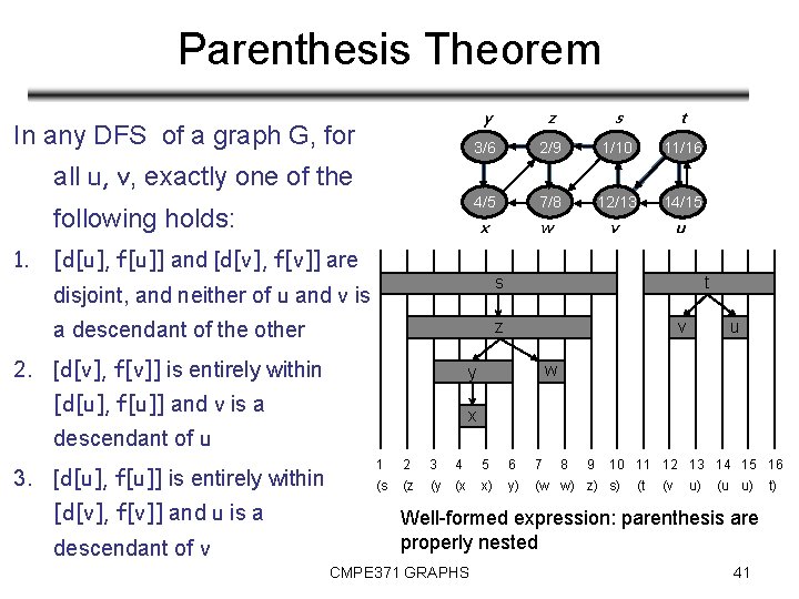
Parenthesis Theorem In any DFS of a graph G, for all u, v, exactly one of the following holds: 1. y z s t 3/6 2/9 1/10 11/16 4/5 7/8 12/13 14/15 x w v u [d[u], f[u]] and [d[v], f[v]] are disjoint, and neither of u and v is s a descendant of the other z 2. [d[v], f[v]] is entirely within descendant of v u w x descendant of u [d[v], f[v]] and u is a v y [d[u], f[u]] and v is a 3. [d[u], f[u]] is entirely within t 1 2 3 4 5 6 7 8 9 10 11 12 13 14 15 16 (s (z (y (x x) y) (w w) z) s) (t (v u) (u u) Well-formed expression: parenthesis are properly nested CMPE 371 GRAPHS 41 t)

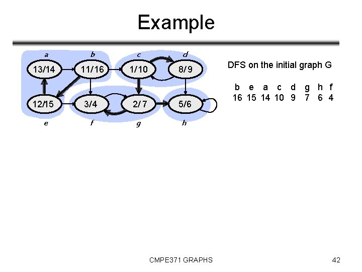
Example a b c d 13/14 11/ 16 1/ 10 8/ 9 12/15 e 3/ 4 2/ 7 5/ 6 f g h CMPE 371 GRAPHS DFS on the initial graph G b e a c d g h f 16 15 14 10 9 7 6 4 42

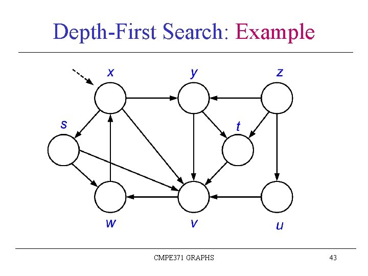
Depth-First Search: Example CMPE 371 GRAPHS 43

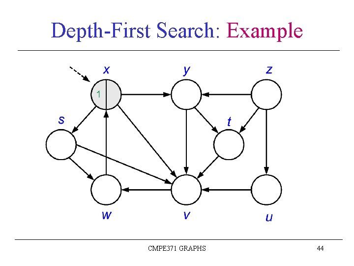
Depth-First Search: Example CMPE 371 GRAPHS 44

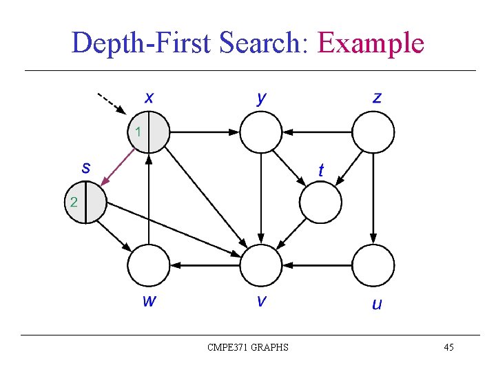
Depth-First Search: Example CMPE 371 GRAPHS 45

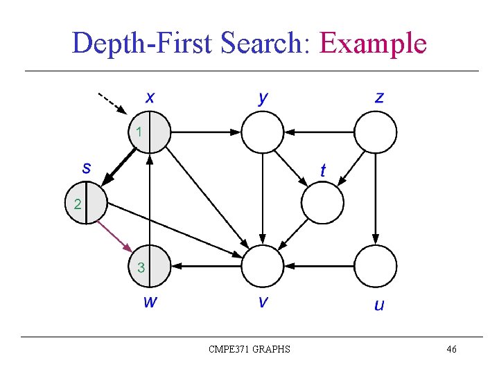
Depth-First Search: Example CMPE 371 GRAPHS 46

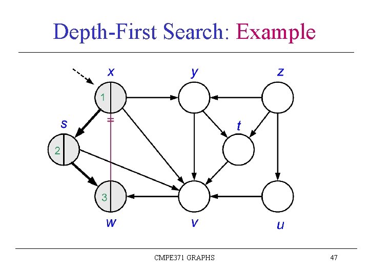
Depth-First Search: Example CMPE 371 GRAPHS 47

Depth-First Search: Example CMPE 371 GRAPHS 48

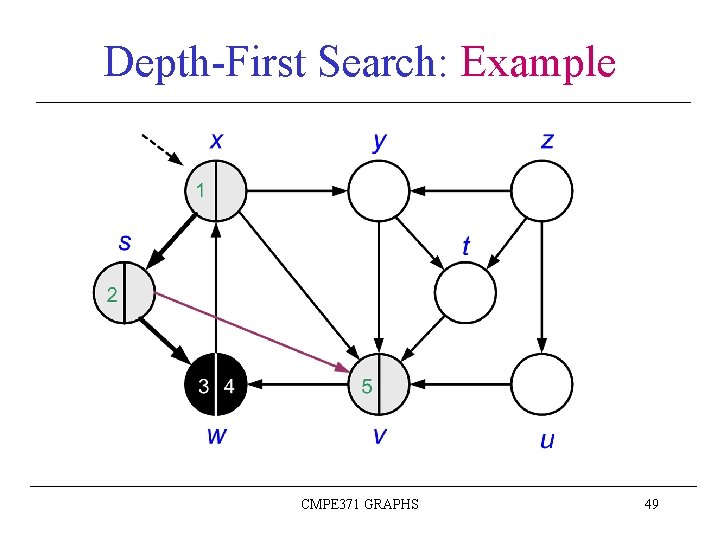
Depth-First Search: Example CMPE 371 GRAPHS 49

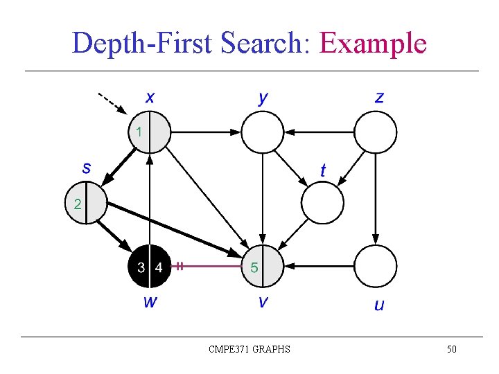
Depth-First Search: Example CMPE 371 GRAPHS 50

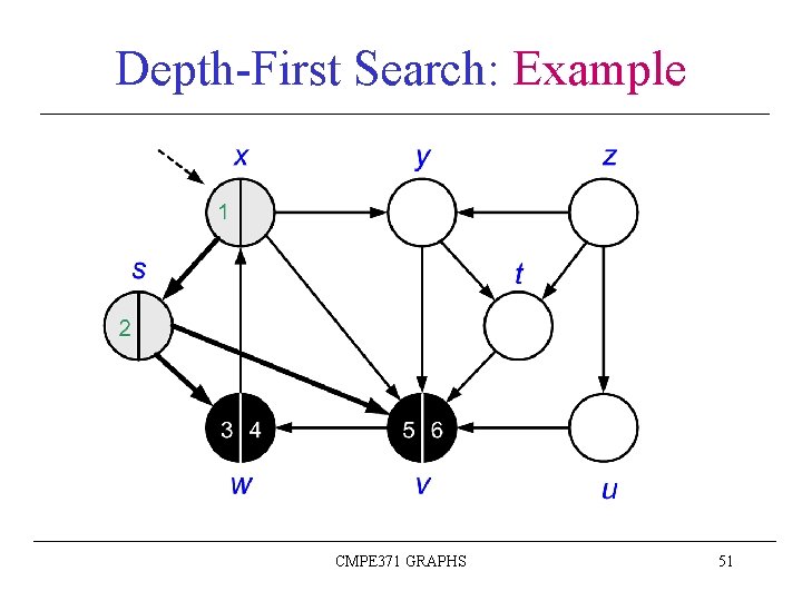
Depth-First Search: Example CMPE 371 GRAPHS 51

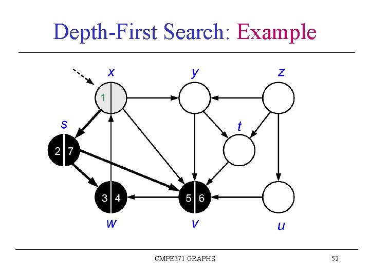
Depth-First Search: Example CMPE 371 GRAPHS 52

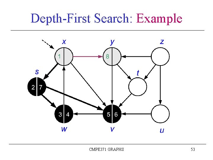
Depth-First Search: Example CMPE 371 GRAPHS 53

Depth-First Search: Example CMPE 371 GRAPHS 54

Depth-First Search: Example CMPE 371 GRAPHS 55

Depth-First Search: Example CMPE 371 GRAPHS 56

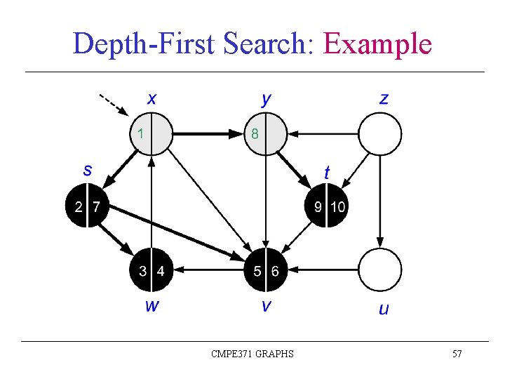
Depth-First Search: Example CMPE 371 GRAPHS 57

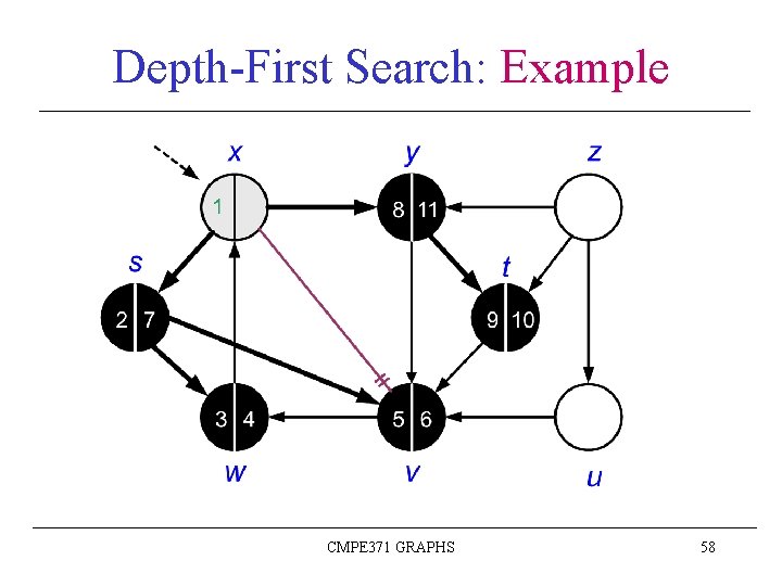
Depth-First Search: Example CMPE 371 GRAPHS 58

Depth-First Search: Example CMPE 371 GRAPHS 59

Depth-First Search: Example CMPE 371 GRAPHS 60

Depth-First Search: Example CMPE 371 GRAPHS 61

Depth-First Search: Example CMPE 371 GRAPHS 62

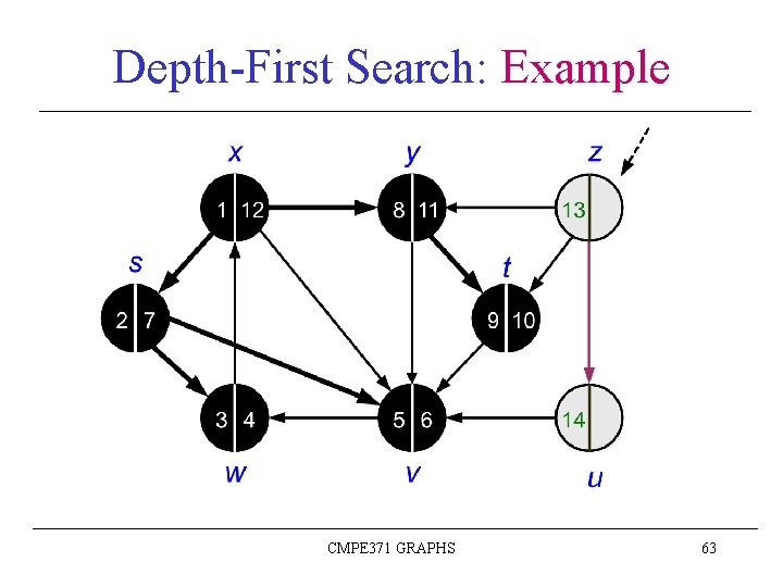
Depth-First Search: Example CMPE 371 GRAPHS 63

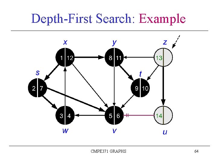
Depth-First Search: Example CMPE 371 GRAPHS 64

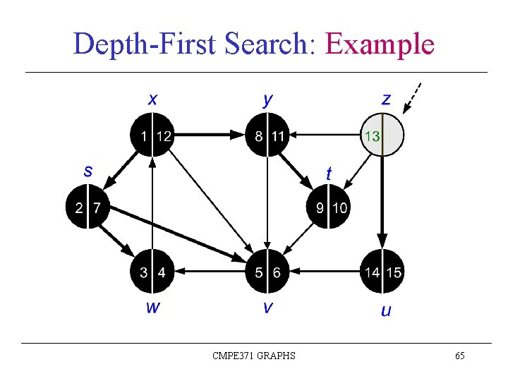
Depth-First Search: Example CMPE 371 GRAPHS 65

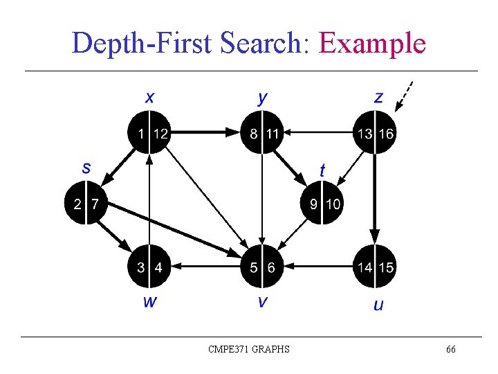
Depth-First Search: Example CMPE 371 GRAPHS 66

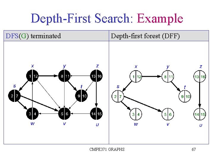
Depth-First Search: Example DFS(G) terminated Depth-first forest (DFF) CMPE 371 GRAPHS 67

MST – Minimum Spanning Tree What greedy algorithm might we use assuming we start with the entire graph l Iteratively take away the biggest remaining link in the graph which does not disconnect the graph l – Is it a greedy approach? l How do we prove if it works or not – Counterexamples – natural first attempt – If no easily found counterexamples, we then seek a more formal proof CS 312 – Greedy Algorithms 68

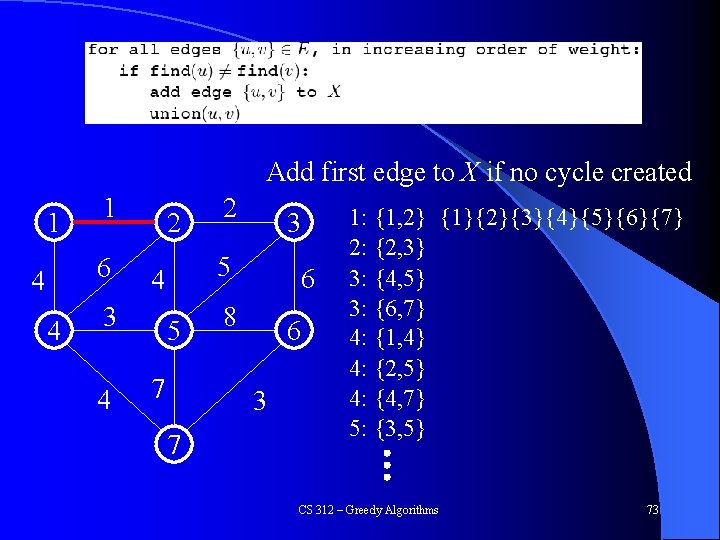
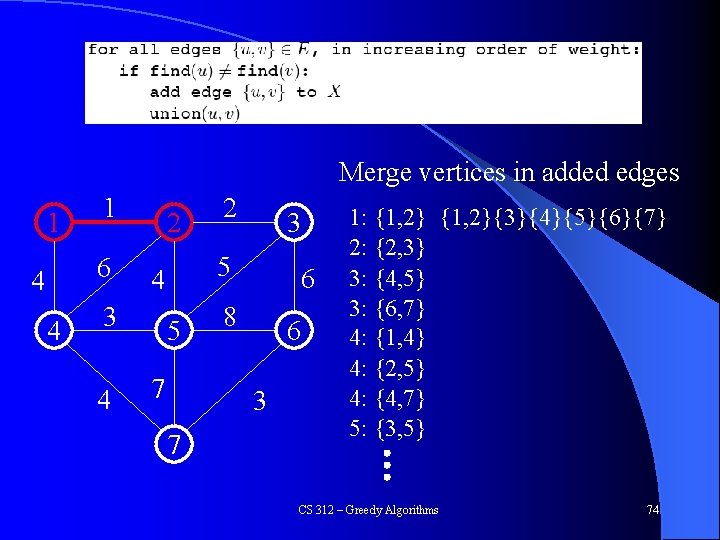
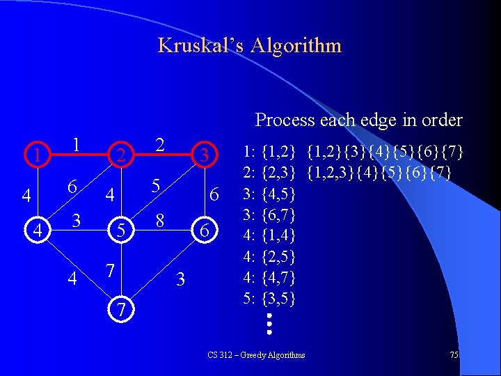
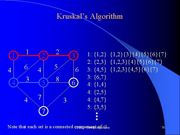
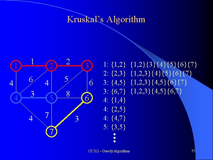
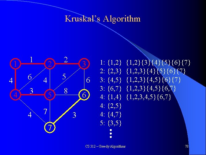
Kruskal's Algorithm Sometimes greedy algorithms can also be optimal! l Kruskal's is a simple greedy optimal algorithm for MST 1. Start with an empty graph 2. Repeatedly add the next smallest edge from E that does not produce a cycle l l How might we test for cycles and what would the complexity be? – more efficient data structure? CS 312 – Greedy Algorithms 69

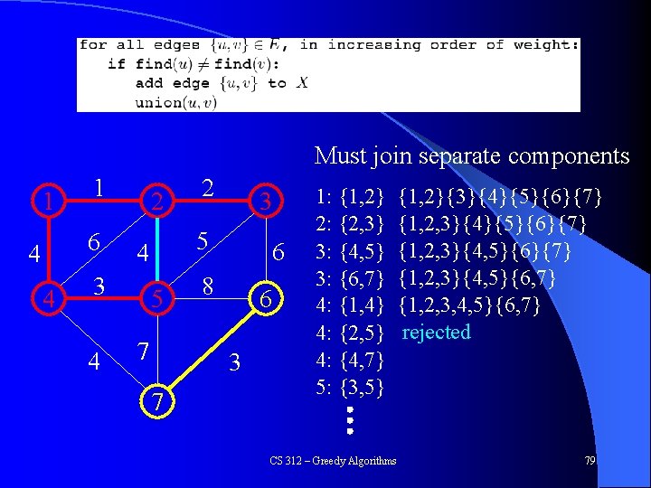
Kruskal's Algorithm Represents nodes in disjoint sets makeset(u): create a singleton set containing just u find(u): to which set does u belong? union(u, v): merge the sets containing u and v CS 312 – Greedy Algorithms find(u) = find(v) if u and v are in the same set, which means they are in the same connected component Why not union nodes that are already in the same set? 70

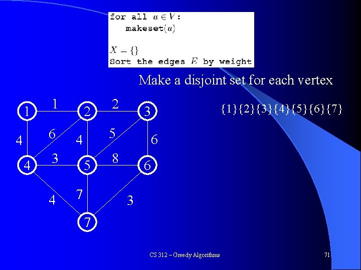
Kruskal’s Algorithm Make a disjoint set for each vertex 1 1 6 4 4 2 4 5 7 {1}{2}{3}{4}{5}{6}{7} 3 5 4 3 2 6 8 6 3 7 CS 312 – Greedy Algorithms 71

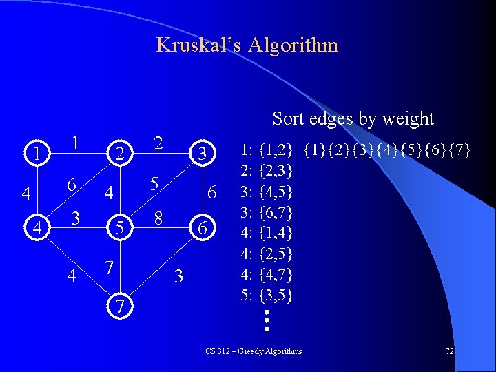
Kruskal’s Algorithm Sort edges by weight 1 1 6 4 4 2 4 3 5 4 3 2 5 7 6 8 6 3 7 1: {1, 2} {1}{2}{3}{4}{5}{6}{7} 2: {2, 3} 3: {4, 5} 3: {6, 7} 4: {1, 4} 4: {2, 5} 4: {4, 7} 5: {3, 5} CS 312 – Greedy Algorithms 72

Kruskal’s Algorithm Add first edge to X if no cycle created 1 1 6 4 4 2 4 3 5 4 3 2 5 7 6 8 6 3 7 1: {1, 2} {1}{2}{3}{4}{5}{6}{7} 2: {2, 3} 3: {4, 5} 3: {6, 7} 4: {1, 4} 4: {2, 5} 4: {4, 7} 5: {3, 5} CS 312 – Greedy Algorithms 73

Kruskal’s Algorithm Merge vertices in added edges 1 1 6 4 4 2 4 3 5 4 3 2 5 7 6 8 6 3 7 1: {1, 2}{3}{4}{5}{6}{7} 2: {2, 3} 3: {4, 5} 3: {6, 7} 4: {1, 4} 4: {2, 5} 4: {4, 7} 5: {3, 5} CS 312 – Greedy Algorithms 74

Kruskal’s Algorithm Process each edge in order 1 1 6 4 4 2 4 3 5 4 3 2 5 7 6 8 6 3 7 1: {1, 2}{3}{4}{5}{6}{7} 2: {2, 3} {1, 2, 3}{4}{5}{6}{7} 3: {4, 5} 3: {6, 7} 4: {1, 4} 4: {2, 5} 4: {4, 7} 5: {3, 5} CS 312 – Greedy Algorithms 75

Kruskal’s Algorithm 1 1 6 4 4 2 4 3 5 4 3 2 5 7 6 8 6 3 7 1: {1, 2}{3}{4}{5}{6}{7} 2: {2, 3} {1, 2, 3}{4}{5}{6}{7} 3: {4, 5} {1, 2, 3}{4, 5}{6}{7} 3: {6, 7} 4: {1, 4} 4: {2, 5} 4: {4, 7} 5: {3, 5} Note that each set is a connected component of G CS 312 – Greedy Algorithms 76

Kruskal’s Algorithm 1 1 6 4 4 2 4 3 5 4 3 2 5 7 6 8 6 3 7 1: {1, 2} 2: {2, 3} 3: {4, 5} 3: {6, 7} 4: {1, 4} 4: {2, 5} 4: {4, 7} 5: {3, 5} {1, 2}{3}{4}{5}{6}{7} {1, 2, 3}{4, 5}{6, 7} CS 312 – Greedy Algorithms 77

Kruskal’s Algorithm 1 1 6 4 4 2 4 3 5 4 3 2 5 7 6 8 6 3 7 1: {1, 2} 2: {2, 3} 3: {4, 5} 3: {6, 7} 4: {1, 4} 4: {2, 5} 4: {4, 7} 5: {3, 5} {1, 2}{3}{4}{5}{6}{7} {1, 2, 3}{4, 5}{6, 7} {1, 2, 3, 4, 5}{6, 7} CS 312 – Greedy Algorithms 78

Kruskal’s Algorithm Must join separate components 1 1 6 4 4 2 4 3 5 4 3 2 5 7 6 8 6 3 7 1: {1, 2} 2: {2, 3} 3: {4, 5} 3: {6, 7} 4: {1, 4} 4: {2, 5} 4: {4, 7} 5: {3, 5} {1, 2}{3}{4}{5}{6}{7} {1, 2, 3}{4, 5}{6, 7} {1, 2, 3, 4, 5}{6, 7} rejected CS 312 – Greedy Algorithms 79

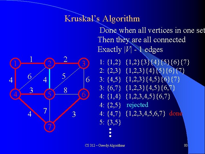
Kruskal’s Algorithm Done when all vertices in one set Then they are all connected Exactly |V| - 1 edges 1 1 6 4 4 2 4 3 5 4 3 2 5 7 6 8 6 3 7 1: {1, 2} 2: {2, 3} 3: {4, 5} 3: {6, 7} 4: {1, 4} 4: {2, 5} 4: {4, 7} 5: {3, 5} {1, 2}{3}{4}{5}{6}{7} {1, 2, 3}{4, 5}{6, 7} {1, 2, 3, 4, 5}{6, 7} rejected {1, 2, 3, 4, 5, 6, 7} done CS 312 – Greedy Algorithms 80

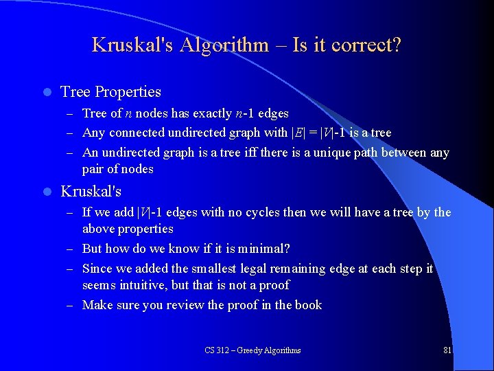
Kruskal's Algorithm – Is it correct? l Tree Properties – Tree of n nodes has exactly n-1 edges – Any connected undirected graph with |E| = |V|-1 is a tree – An undirected graph is a tree iff there is a unique path between any pair of nodes l Kruskal's – If we add |V|-1 edges with no cycles then we will have a tree by the above properties – But how do we know if it is minimal? – Since we added the smallest legal remaining edge at each step it seems intuitive, but that is not a proof – Make sure you review the proof in the book CS 312 – Greedy Algorithms 81