Analysis of Algorithms Chapter 07 Dynamic Programming 1

Analysis of Algorithms Chapter - 07 Dynamic Programming 1

This Chapter Contains the following Topics: 1. Introduction i. What is Dynamic Programming? ii. Elements of Dynamic Programming 2. Matrix-Chain Multiplication i. Matrix-Chain Multiplication Problem ii. Algorithms iii. Examples 2

Introduction 3

What is Dynamic Programming? Ø Dynamic programming solves optimization problems by combining solutions to subproblems. Ø “Programming” refers to a tabular method with a series of choices, not “coding” Ø A set of choices must be made to arrive at an optimal solution. Ø As choices are made, subproblems of the same form arise frequently. Ø The key is to store the solutions of subproblems to be reused in the future. Ø Recall the divide-and-conquer approach: Ø Partition the problem into independent subproblems. Ø Solve the subproblems recursively. Ø Combine solutions of subproblems. Ø This contrasts with the dynamic programming approach. 4

What is Dynamic Programming? Ø Dynamic programming is applicable when subproblems are not independent. Ø i. e. , subproblems share subsubproblems Ø Solve every subsubproblem only once and store the answer for use when it reappears. Ø A divide-and-conquer approach will do more work than necessary. Ø A dynamic programming approach consists of a sequence of 4 steps: Ø Characterize the structure of an optimal solution. Ø Recursively define the value of an optimal solution. Ø Compute the value of an optimal solution in a bottom-up fashion. Ø Construct an optimal solution from computed information 5

Elements of Dynamic Programming Ø For dynamic programming to be applicable, an optimization problem must have: Ø Optimal substructure Ø An optimal solution to the problem contains within it optimal solution to subproblems (but this may also mean a greedy strategy applies) Ø Overlapping subproblems Ø The space of subproblems must be small; i. e. , the same subproblems are encountered over and over 6

Matrix-Chain Multiplication 7

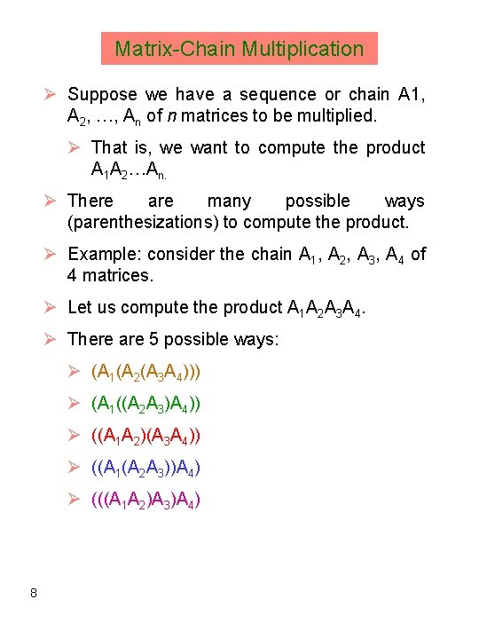
Matrix-Chain Multiplication Ø Suppose we have a sequence or chain A 1, A 2, …, An of n matrices to be multiplied. Ø That is, we want to compute the product A 1 A 2…An. Ø There are many possible ways (parenthesizations) to compute the product. Ø Example: consider the chain A 1, A 2, A 3, A 4 of 4 matrices. Ø Let us compute the product A 1 A 2 A 3 A 4. Ø There are 5 possible ways: Ø (A 1(A 2(A 3 A 4))) Ø (A 1((A 2 A 3)A 4)) Ø ((A 1 A 2)(A 3 A 4)) Ø ((A 1(A 2 A 3))A 4) Ø (((A 1 A 2)A 3)A 4) 8

Multiplication of Two Matrices Ø To compute the number of scalar multiplications necessary, we must know: Ø Algorithm to multiply two matrices. Ø Matrix dimensions. Ø Input: Matrices Ap×q and Bq×r Ø Output: Matrix Cp×r resulting from A·B Algorithm Matrix-Multiply(Ap×q , Bq×r) { for i : = 1 to p do for j : = 1 to r do { C[i, j] : = 0; for k : = 1 to q do C[i, j] : = C[i, j] + A[i, k] · B[k, j]; } return C; } Ø Number of scalar multiplications = pqr 9

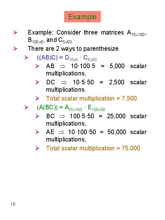
Example Ø Example: Consider three matrices A 10 100, B 100 5, and C 5 50 Ø There are 2 ways to parenthesize Ø ((AB)C) = D 10 5 · C 5 50 Ø AB 10· 100· 5 = 5, 000 scalar multiplications, Ø DC 10· 5· 50 = 2, 500 scalar multiplications, Ø Total scalar multiplication = 7, 500 Ø (A(BC)) = A 10 100 · E 100 50 Ø BC 100· 5· 50 = 25, 000 scalar multiplications, Ø AE 10· 100· 50 = 50, 000 scalar multiplications, Ø Total scalar multiplication = 75, 000 10

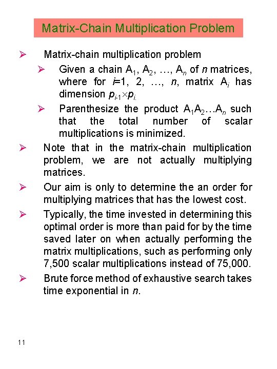
Matrix-Chain Multiplication Problem Ø Ø Ø 11 Matrix-chain multiplication problem Ø Given a chain A 1, A 2, …, An of n matrices, where for i=1, 2, …, n, matrix Ai has dimension pi-1 pi. Ø Parenthesize the product A 1 A 2…An such that the total number of scalar multiplications is minimized. Note that in the matrix-chain multiplication problem, we are not actually multiplying matrices. Our aim is only to determine the an order for multiplying matrices that has the lowest cost. Typically, the time invested in determining this optimal order is more than paid for by the time saved later on when actually performing the matrix multiplications, such as performing only 7, 500 scalar multiplications instead of 75, 000. Brute force method of exhaustive search takes time exponential in n.

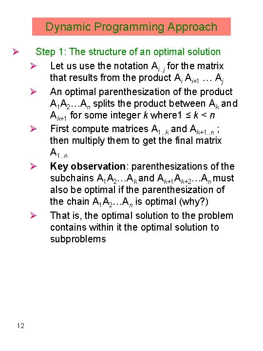
Dynamic Programming Approach Ø 12 Step 1: The structure of an optimal solution Ø Let us use the notation Ai. . j for the matrix that results from the product Ai Ai+1 … Aj Ø An optimal parenthesization of the product A 1 A 2…An splits the product between Ak and Ak+1 for some integer k where 1 ≤ k < n Ø First compute matrices A 1. . k and Ak+1. . n ; then multiply them to get the final matrix A 1. . n Ø Key observation: parenthesizations of the subchains A 1 A 2…Ak and Ak+1 Ak+2…An must also be optimal if the parenthesization of the chain A 1 A 2…An is optimal (why? ) Ø That is, the optimal solution to the problem contains within it the optimal solution to subproblems

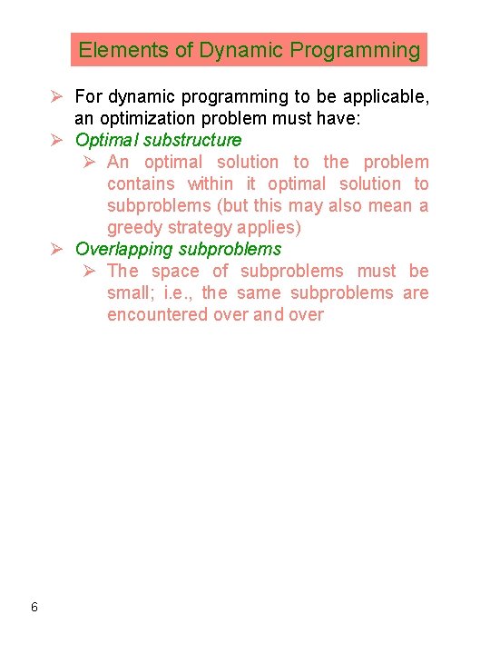
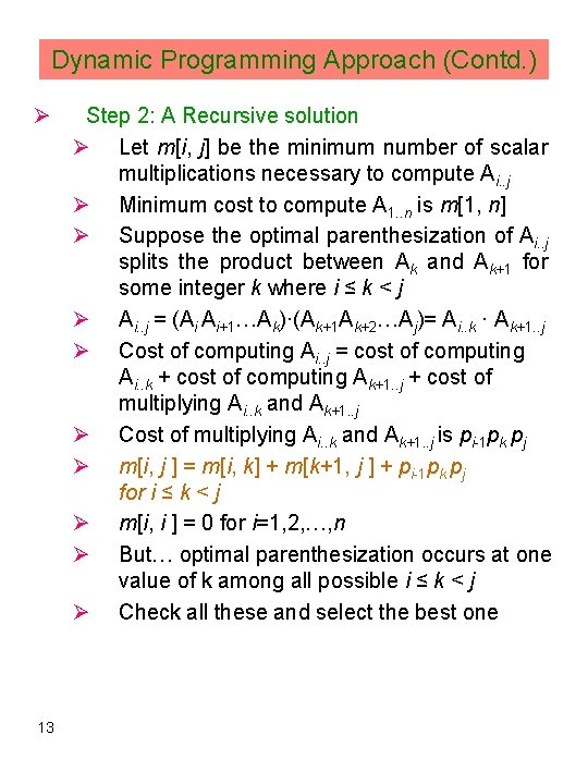
Dynamic Programming Approach (Contd. ) Ø 13 Step 2: A Recursive solution Ø Let m[i, j] be the minimum number of scalar multiplications necessary to compute Ai. . j Ø Minimum cost to compute A 1. . n is m[1, n] Ø Suppose the optimal parenthesization of Ai. . j splits the product between Ak and Ak+1 for some integer k where i ≤ k < j Ø Ai. . j = (Ai Ai+1…Ak)·(Ak+1 Ak+2…Aj)= Ai. . k · Ak+1. . j Ø Cost of computing Ai. . j = cost of computing Ai. . k + cost of computing Ak+1. . j + cost of multiplying Ai. . k and Ak+1. . j Ø Cost of multiplying Ai. . k and Ak+1. . j is pi-1 pk pj Ø m[i, j ] = m[i, k] + m[k+1, j ] + pi-1 pk pj for i ≤ k < j Ø m[i, i ] = 0 for i=1, 2, …, n Ø But… optimal parenthesization occurs at one value of k among all possible i ≤ k < j Ø Check all these and select the best one

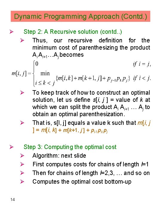
Dynamic Programming Approach (Contd. ) Ø Step 2: A Recursive solution (contd. . ) Ø Thus, our recursive definition for the minimum cost of parenthesizing the product Ai Ai+1…Aj becomes Ø Ø Ø 14 To keep track of how to construct an optimal solution, let us define s[i, j ] = value of k at which we can split the product Ai Ai+1 … Aj to obtain an optimal parenthesization. That is, s[I, j] equals a value k such that m[i, j ] = m[i, k] + m[k+1, j ] + pi-1 pk pj Step 3: Computing the optimal cost Ø Algorithm: next slide Ø First computes costs for chains of length l=1 Ø Then for chains of length l=2, 3, … and so on Ø Computes the optimal cost bottom-up

Dynamic Programming Approach (Contd. ) Ø Input: Array p[0…n] containing matrix dimensions and n Ø Result: Minimum-cost table m and split table s Algorithm Matrix. Chain. Order(p[ ], n) { for i : = 1 to n do m[i, i] : = 0; for l : = 2 to n do for i : = 1 to n-l+1 do { j : = i+l-1; m[i, j] : = ; for k : = i to j-1 do { q : = m[i, k] + m[k+1, j] + p[i-1] p[k] p[j]; if (q < m[i, j]) then { m[i, j] : = q; s[i, j] : = k; } } return m and s } 15

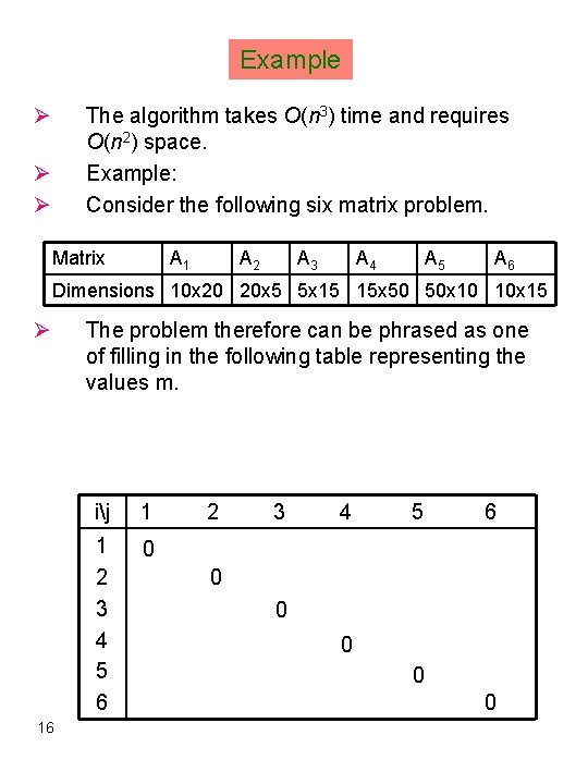
Example Ø The algorithm takes O(n 3) time and requires O(n 2) space. Example: Consider the following six matrix problem. Ø Ø Matrix A 1 A 2 A 3 A 4 A 5 A 6 Dimensions 10 x 20 20 x 5 5 x 15 15 x 50 50 x 10 10 x 15 Ø 16 The problem therefore can be phrased as one of filling in the following table representing the values m. ij 1 1 2 3 4 5 6 0 0 0

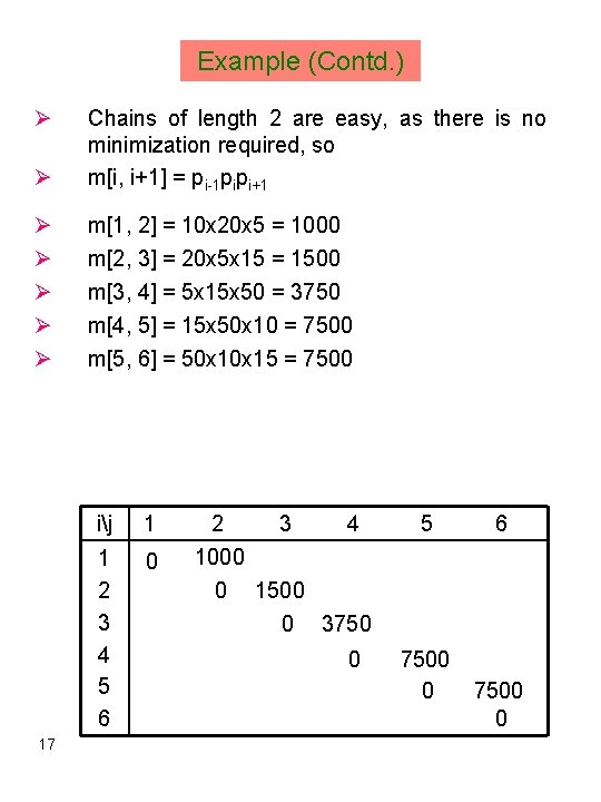
Example (Contd. ) Ø Ø Chains of length 2 are easy, as there is no minimization required, so m[i, i+1] = pi-1 pipi+1 Ø Ø Ø m[1, 2] = 10 x 20 x 5 = 1000 m[2, 3] = 20 x 5 x 15 = 1500 m[3, 4] = 5 x 15 x 50 = 3750 m[4, 5] = 15 x 50 x 10 = 7500 m[5, 6] = 50 x 15 = 7500 17 ij 1 1 2 3 4 5 6 0 2 3 4 1000 0 1500 0 3750 0 5 7500 0 6 7500 0

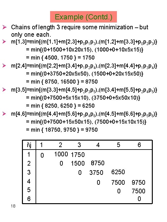
Example (Contd. ) Ø Chains of length 3 require some minimization – but only one each. Ø m[1, 3]=min{(m[1, 1]+m[2, 3]+p 0 p 1 p 3), (m[1, 2]+m[3, 3]+p 0 p 2 p 3)} = min{(0+1500+10 x 20 x 15), (1000+0+10 x 5 x 15)} = min { 4500, 1750 } = 1750 Ø m[2, 4]=min{(m[2, 2]+m[3, 4]+p 1 p 2 p 4), (m[2, 3]+m[4, 4]+p 1 p 3 p 4)} = min{(0+3750+20 x 5 x 50), (1500+0+20 x 15 x 50)} = min { 8750, 16500 } = 8750 Ø m[3, 5]=min{(m[3, 3]+m[4, 5]+p 2 p 3 p 5), (m[3, 4]+m[5, 5]+p 2 p 4 p 5)} = min{(0+7500+5 x 10), (3750+0+5 x 50 x 10)} = min { 8250, 6250 } = 6250 Ø m[4, 6]=min{(m[4, 4]+m[5, 6]+p 3 p 4 p 6), (m[4, 5]+m[6, 6]+p 3 p 5 p 6)} = min{(0+7500+15 x 50 x 15), (7500+0+15 x 10 x 15)} = min { 18750, 9750 } = 9750 18 ij 1 1 2 3 4 5 6 0 2 3 4 1000 1750 0 1500 8750 0 3750 0 5 6 6250 7500 0 9750 7500 0

Example (Contd. ) Ø m[1, 4]=min{(m[1, 1]+m[2, 4]+p 0 p 1 p 4), (m[1, 2]+m[3, 4]+p 0 p 2 p 4), (m[1, 3]+m[4, 4]+p 0 p 3 p 4)} = min{(0+8750+10 x 20 x 50), (1000+3750+10 x 5 x 50), (1750+0+10 x 15 x 50)} = min { 18750, 7250, 9250 } = 7250 Ø m[2, 5]=min{(m[2, 2]+m[3, 5]+p 1 p 2 p 5), (m[2, 3]+m[4, 5]+p 1 p 3 p 5), (m[2, 4]+m[5, 5]+p 1 p 4 p 5)} = min{(0+6250+20 x 5 x 10), (1500+7500+20 x 15 x 10), (8750+0+20 x 50 x 10)} = min { 7250, 12000, 18750 } = 7250 Ø m[3, 6]=min{(m[3, 3]+m[4, 6]+p 2 p 3 p 6), (m[3, 4]+m[5, 6]+p 2 p 4 p 6), (m[3, 5]+m[6, 6]+p 2 p 5 p 6)} = min{(0+9750+5 x 15), (3750+7500+5 x 50 x 15), (6250+0+5 x 10 x 15)} = min { 10875, 15000, 7000 } = 7000 19 ij 1 1 2 3 4 5 6 0 2 3 4 5 1000 1750 7250 0 1500 8750 7250 0 3750 6250 0 7500 0 6 7000 9750 7500 0

Example (Contd. ) Ø m[1, 5]=min{(m[1, 1]+m[2, 5]+p 0 p 1 p 5), (m[1, 2]+m[3, 5]+p 0 p 2 p 5), (m[1, 3]+m[4, 5]+p 0 p 3 p 5), (m[1, 4]+m[5, 5]+p 0 p 4 p 5)} = min{(0+7250+10 x 20 x 10), (1000+6250+10 x 5 x 10), (1750+7500+10 x 15 x 10), (7250+0+10 x 50 x 10)} = min { 9250, 7750, 10750, 12250 } = 7750 Ø m[2, 6]=min{(m[2, 2]+m[3, 6]+p 1 p 2 p 6), (m[2, 3]+m[4, 6]+p 1 p 3 p 6), (m[2, 4]+m[5, 6]+p 1 p 4 p 6), (m[2, 5]+m[6, 6]+p 1 p 5 p 6)} = min{(0+7000+20 x 5 x 15), (1500+9750+20 x 15), (8750+7500+20 x 50 x 15), (7250+0+20 x 15)} = min { 8500, 15750, 31, 250, 10250 } = 8500 Ø m[1, 6]=min{(m[1, 1]+m[2, 6]+p 0 p 1 p 6), (m[1, 2]+m[3, 6]+p 0 p 2 p 6), (m[1, 3]+m[4, 6]+p 0 p 3 p 6), (m[1, 4]+m[5, 6]+p 0 p 4 p 6), (m[1, 5]+m[6, 6]+p 0 p 5 p 6)} = min{(11500, 8750, 13750, 22250, 9250 } = 8750 20 ij 1 1 2 3 4 5 6 0 2 3 4 5 6 1000 1750 7250 7750 8750 0 1500 8750 7250 8500 0 3750 6250 7000 0 7500 0 9750 7500 0

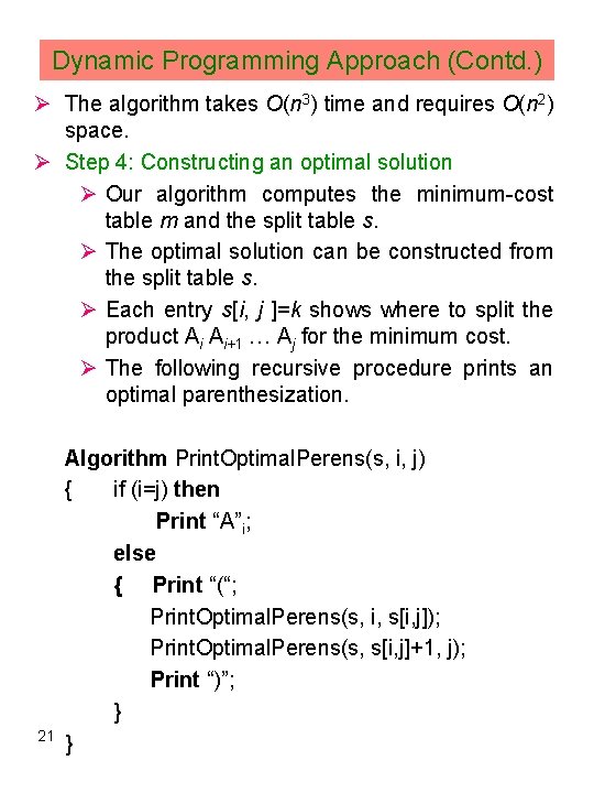
Dynamic Programming Approach (Contd. ) Ø The algorithm takes O(n 3) time and requires O(n 2) space. Ø Step 4: Constructing an optimal solution Ø Our algorithm computes the minimum-cost table m and the split table s. Ø The optimal solution can be constructed from the split table s. Ø Each entry s[i, j ]=k shows where to split the product Ai Ai+1 … Aj for the minimum cost. Ø The following recursive procedure prints an optimal parenthesization. 21 Algorithm Print. Optimal. Perens(s, i, j) { if (i=j) then Print “A”i; else { Print “(“; Print. Optimal. Perens(s, i, s[i, j]); Print. Optimal. Perens(s, s[i, j]+1, j); Print “)”; } }

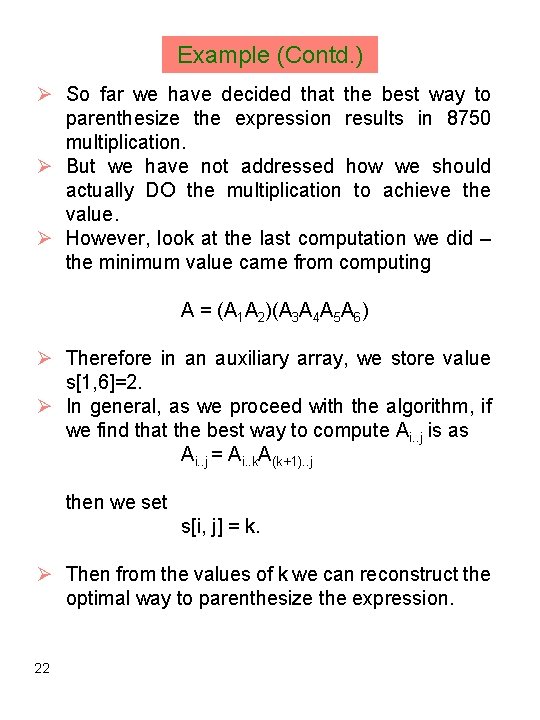
Example (Contd. ) Ø So far we have decided that the best way to parenthesize the expression results in 8750 multiplication. Ø But we have not addressed how we should actually DO the multiplication to achieve the value. Ø However, look at the last computation we did – the minimum value came from computing A = (A 1 A 2)(A 3 A 4 A 5 A 6) Ø Therefore in an auxiliary array, we store value s[1, 6]=2. Ø In general, as we proceed with the algorithm, if we find that the best way to compute Ai. . j is as Ai. . j = Ai. . k. A(k+1). . j then we set s[i, j] = k. Ø Then from the values of k we can reconstruct the optimal way to parenthesize the expression. 22

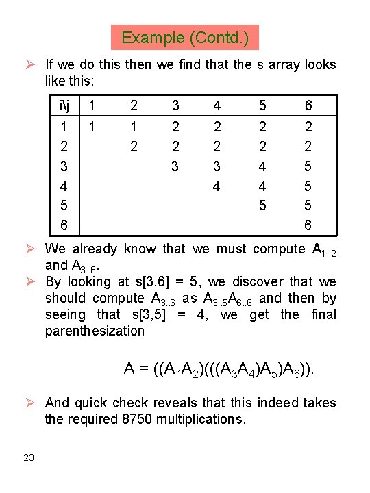
Example (Contd. ) Ø If we do this then we find that the s array looks like this: ij 1 2 3 4 5 6 1 1 2 2 2 3 4 2 2 4 4 5 2 2 5 5 5 6 Ø We already know that we must compute A 1. . 2 and A 3. . 6. Ø By looking at s[3, 6] = 5, we discover that we should compute A 3. . 6 as A 3. . 5 A 6. . 6 and then by seeing that s[3, 5] = 4, we get the final parenthesization A = ((A 1 A 2)(((A 3 A 4)A 5)A 6)). Ø And quick check reveals that this indeed takes the required 8750 multiplications. 23