Analysis of Algorithms b Issues Correctness Time efficiency

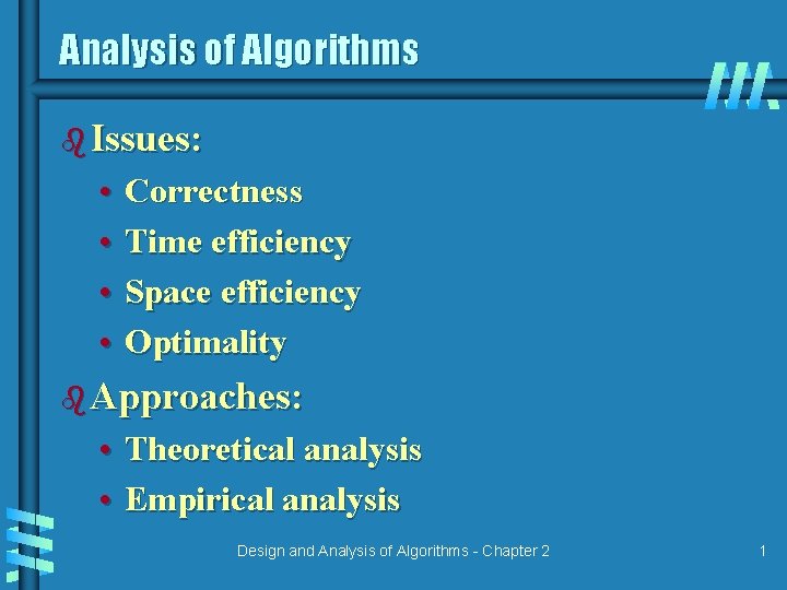
Analysis of Algorithms b Issues: • • Correctness Time efficiency Space efficiency Optimality b Approaches: • Theoretical analysis • Empirical analysis Design and Analysis of Algorithms - Chapter 2 1

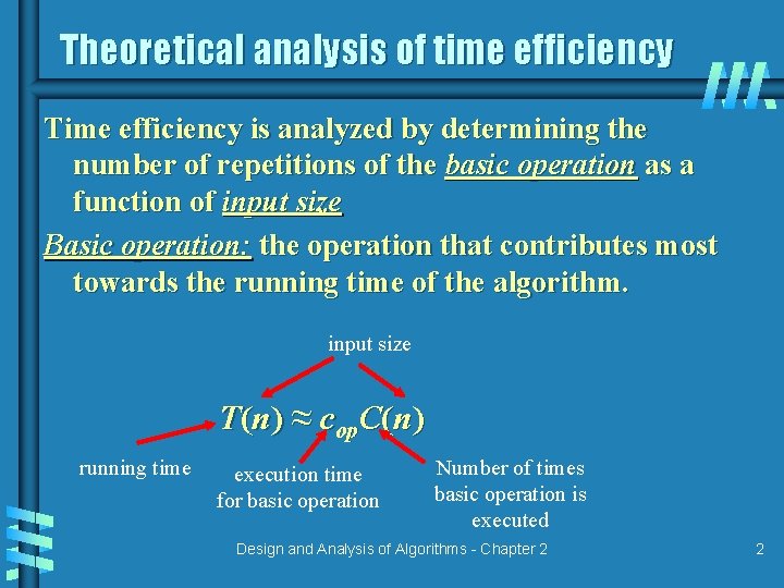
Theoretical analysis of time efficiency Time efficiency is analyzed by determining the number of repetitions of the basic operation as a function of input size Basic operation: the operation that contributes most towards the running time of the algorithm. input size T(n) ≈ cop. C(n) running time execution time for basic operation Number of times basic operation is executed Design and Analysis of Algorithms - Chapter 2 2

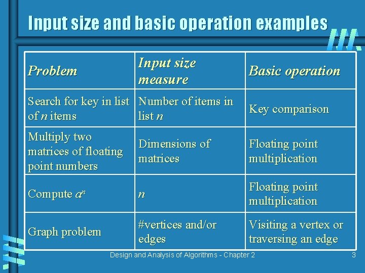
Input size and basic operation examples Input size measure Problem Basic operation Search for key in list Number of items in of n items list n Key comparison Multiply two matrices of floating point numbers Dimensions of matrices Floating point multiplication Compute an n Floating point multiplication Graph problem #vertices and/or edges Visiting a vertex or traversing an edge Design and Analysis of Algorithms - Chapter 2 3

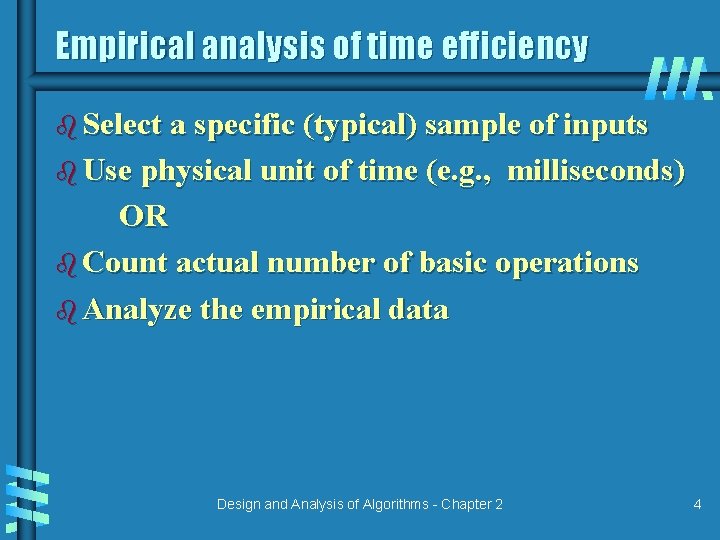
Empirical analysis of time efficiency b Select a specific (typical) sample of inputs b Use physical unit of time (e. g. , milliseconds) OR b Count actual number of basic operations b Analyze the empirical data Design and Analysis of Algorithms - Chapter 2 4

Best-case, average-case, worst-case For some algorithms efficiency depends on type of input: b Worst case: W(n) – maximum over inputs of size n b Best case: B(n) – minimum over inputs of size n b Average case: A(n) – “average” over inputs of size n • Number of times the basic operation will be executed on typical input • NOT the average of worst and best case • Expected number of basic operations repetitions considered as a random variable under some assumption about the probability distribution of all possible inputs of size n Design and Analysis of Algorithms - Chapter 2 5

Example: Sequential search b Problem: Given a list of n elements and a search key K, find an element equal to K, if any. b Algorithm: Scan the list and compare its successive elements with K until either a matching element is found (successful search) or the list is exhausted (unsuccessful search) b Worst case b Best case b Average case Design and Analysis of Algorithms - Chapter 2 6

Types of formulas for basic operation count b Exact formula e. g. , C(n) = n(n-1)/2 b Formula indicating order of growth with specific multiplicative constant e. g. , C(n) ≈ 0. 5 n 2 b Formula indicating order of growth with unknown multiplicative constant e. g. , C(n) ≈ cn 2 Design and Analysis of Algorithms - Chapter 2 7

Order of growth b Most important: Order of growth within a constant multiple as n→∞ b Example: • How much faster will algorithm run on computer that is twice as fast? • How much longer does it take to solve problem of double input size? b See table 2. 1 Design and Analysis of Algorithms - Chapter 2 8

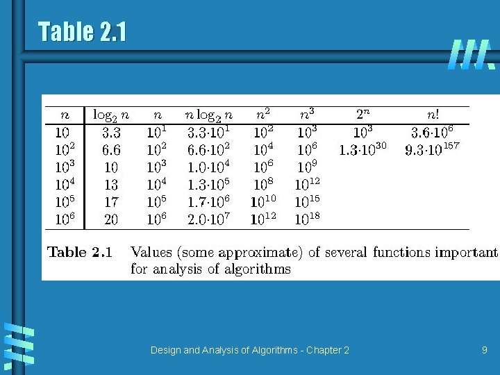
Table 2. 1 Design and Analysis of Algorithms - Chapter 2 9

Asymptotic growth rate b A way of comparing functions that ignores constant factors and small input sizes b O(g(n)): class of functions f(n) that grow no faster than g(n) b Θ(g(n)): class of functions f(n) that grow at same rate as g(n) b Ω(g(n)): class of functions f(n) that grow at least as fast as g(n) see figures 2. 1, 2. 2, 2. 3 Design and Analysis of Algorithms - Chapter 2 10

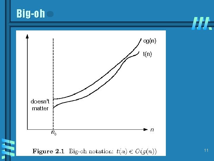
Big-oh Design and Analysis of Algorithms - Chapter 2 11

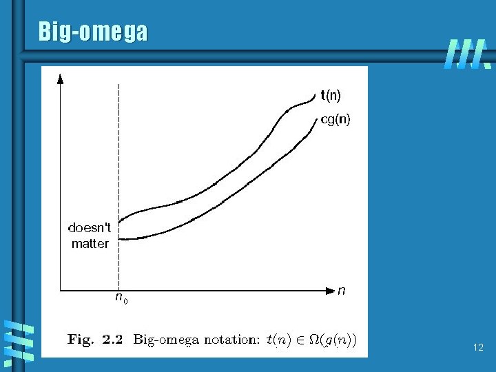
Big-omega Design and Analysis of Algorithms - Chapter 2 12

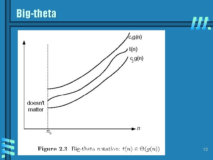
Big-theta Design and Analysis of Algorithms - Chapter 2 13

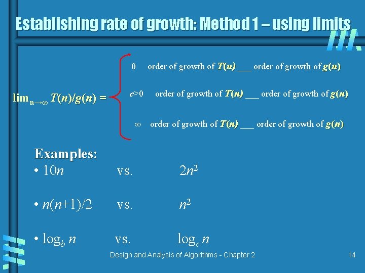
Establishing rate of growth: Method 1 – using limits 0 limn→∞ T(n)/g(n) = c>0 ∞ order of growth of T(n) ___ order of growth of g(n) Examples: • 10 n vs. 2 n 2 • n(n+1)/2 vs. n 2 • logb n vs. logc n Design and Analysis of Algorithms - Chapter 2 14

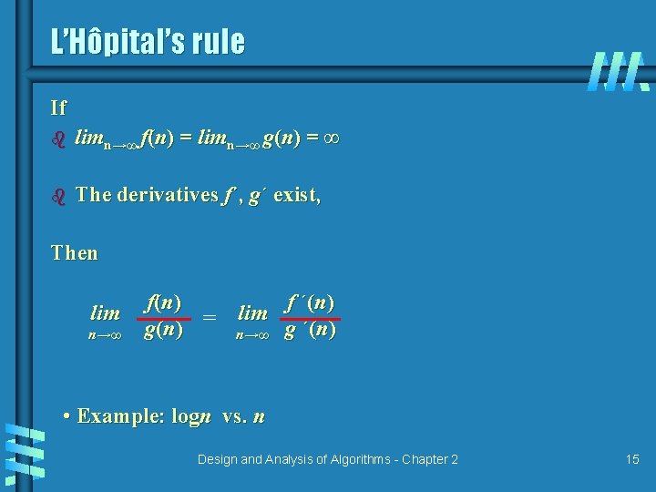
L’Hôpital’s rule If b limn→∞ f(n) = limn→∞ g(n) = ∞ b The derivatives f´, g´ exist, Then lim n→∞ f(n ) g(n) = lim f ´(n) n→∞ g ´(n) • Example: logn vs. n Design and Analysis of Algorithms - Chapter 2 15

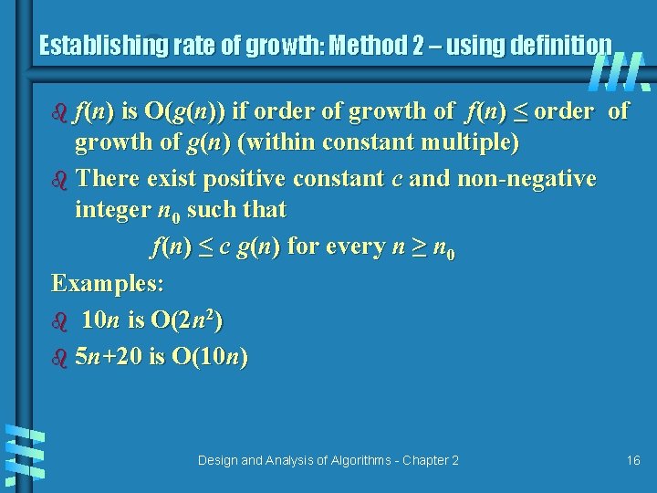
Establishing rate of growth: Method 2 – using definition b f(n) is O(g(n)) if order of growth of f(n) ≤ order of growth of g(n) (within constant multiple) b There exist positive constant c and non-negative integer n 0 such that f(n) ≤ c g(n) for every n ≥ n 0 Examples: b 10 n is O(2 n 2) b 5 n+20 is O(10 n) Design and Analysis of Algorithms - Chapter 2 16

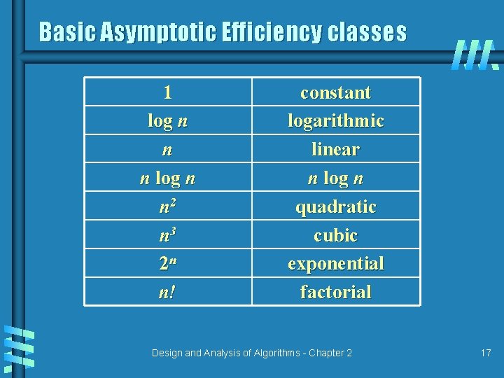
Basic Asymptotic Efficiency classes 1 log n n n log n n 2 n 3 2 n n! constant logarithmic linear n log n quadratic cubic exponential factorial Design and Analysis of Algorithms - Chapter 2 17

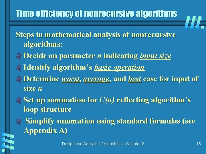
Time efficiency of nonrecursive algorithms Steps in mathematical analysis of nonrecursive algorithms: b Decide on parameter n indicating input size b Identify algorithm’s basic operation b Determine worst, average, and best case for input of size n b Set up summation for C(n) reflecting algorithm’s loop structure b Simplify summation using standard formulas (see Appendix A) Design and Analysis of Algorithms - Chapter 2 18

A simple example Algorithm Max. Element(A[0. . n-1]) // Determines the value of the largest element in a given array // Input: An array A[0. . n-1] of real numbers // Output: The value of the largest element in A maxval A[0] for i 1 to n-1 do if A[i]>maxval A[i] return maxval Design and Analysis of Algorithms - Chapter 2 19

Another simple example Algorithm Unique. Element(A[0. . n-1]) // Check whether all the elements in a array are distinct // Input: An array A[0. . n-1] of real numbers // Output: Returns “true” if all the elements are distinct for i 0 to n-2 do for j i+1 to n-1 do if A[i]=A[j] return false return true Design and Analysis of Algorithms - Chapter 2 20

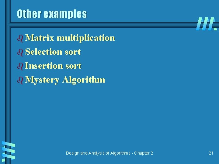
Other examples b Matrix multiplication b Selection sort b Insertion sort b Mystery Algorithm Design and Analysis of Algorithms - Chapter 2 21

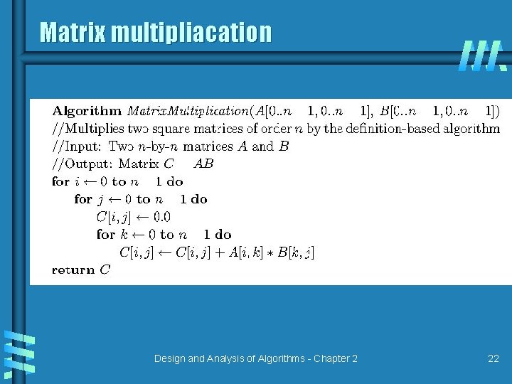
Matrix multipliacation Design and Analysis of Algorithms - Chapter 2 22

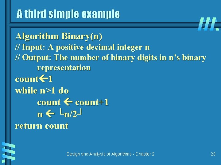
A third simple example Algorithm Binary(n) // Input: A positive decimal integer n // Output: The number of binary digits in n’s binary representation count 1 while n>1 do count+1 n └n/2┘ return count Design and Analysis of Algorithms - Chapter 2 23

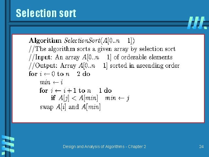
Selection sort Design and Analysis of Algorithms - Chapter 2 24

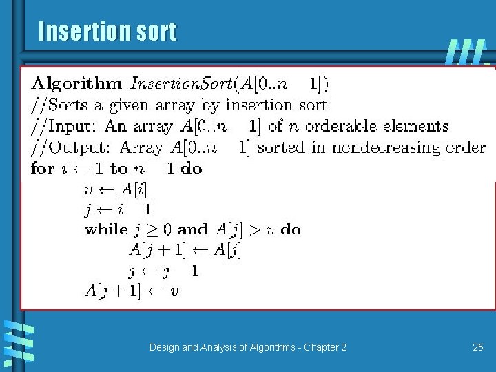
Insertion sort Design and Analysis of Algorithms - Chapter 2 25

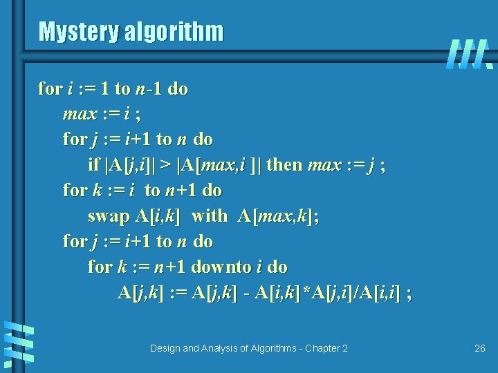
Mystery algorithm for i : = 1 to n-1 do max : = i ; for j : = i+1 to n do if |A[j, i]| > |A[max, i ]| then max : = j ; for k : = i to n+1 do swap A[i, k] with A[max, k]; for j : = i+1 to n do for k : = n+1 downto i do A[j, k] : = A[j, k] - A[i, k]*A[j, i]/A[i, i] ; Design and Analysis of Algorithms - Chapter 2 26

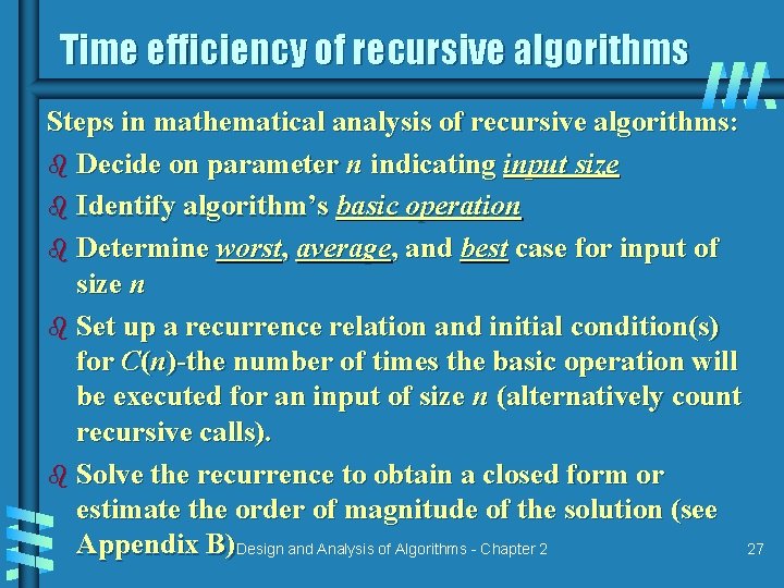
Time efficiency of recursive algorithms Steps in mathematical analysis of recursive algorithms: b Decide on parameter n indicating input size b Identify algorithm’s basic operation b Determine worst, average, and best case for input of size n b Set up a recurrence relation and initial condition(s) for C(n)-the number of times the basic operation will be executed for an input of size n (alternatively count recursive calls). b Solve the recurrence to obtain a closed form or estimate the order of magnitude of the solution (see Appendix B)Design and Analysis of Algorithms - Chapter 2 27

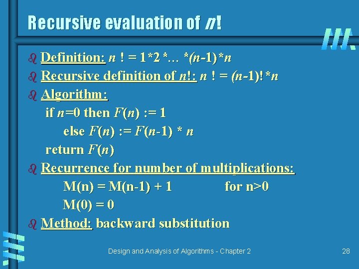
Recursive evaluation of n ! b Definition: n ! = 1*2*…*(n-1)*n b Recursive definition of n!: n ! = (n-1)!*n b Algorithm: if n=0 then F(n) : = 1 else F(n) : = F(n-1) * n return F(n) b Recurrence for number of multiplications: M(n) = M(n-1) + 1 for n>0 M(0) = 0 b Method: backward substitution Design and Analysis of Algorithms - Chapter 2 28

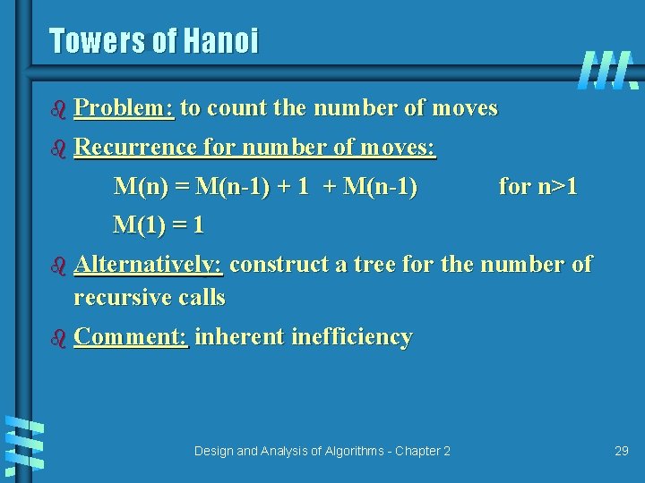
Towers of Hanoi b Problem: to count the number of moves b Recurrence for number of moves: M(n) = M(n-1) + 1 + M(n-1) for n>1 M(1) = 1 b Alternatively: construct a tree for the number of recursive calls b Comment: inherent inefficiency Design and Analysis of Algorithms - Chapter 2 29

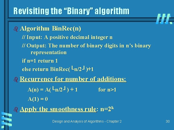
Revisiting the “Binary” algorithm b Algorithm Bin. Rec(n) // Input: A positive decimal integer n // Output: The number of binary digits in n’s binary representation if n=1 return 1 else return Bin. Rec(└n/2┘)+1 b Recurrence for number of additions: A(n) = A(└n/2┘) + 1 for n>1 A(1) = 0 b Apply the smoothness rule: n=2 k Design and Analysis of Algorithms - Chapter 2 30

Computing Fibonacci numbers (1) 1. Definition based recursive algorithm 2. Nonrecursive brute-force algorithm 3. Explicit formula algorithm 4. Algorithm based on matrix multiplications Design and Analysis of Algorithms - Chapter 2 31

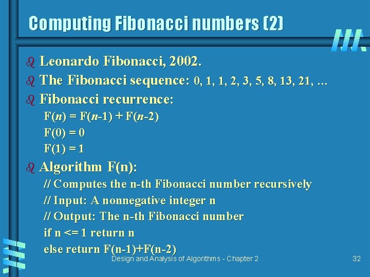
Computing Fibonacci numbers (2) b Leonardo Fibonacci, 2002. b The Fibonacci sequence: 0, 1, 1, 2, 3, 5, 8, 13, 21, … b Fibonacci recurrence: F(n) = F(n-1) + F(n-2) F(0) = 0 F(1) = 1 b Algorithm F(n): // Computes the n-th Fibonacci number recursively // Input: A nonnegative integer n // Output: The n-th Fibonacci number if n <= 1 return n else return F(n-1)+F(n-2) Design and Analysis of Algorithms - Chapter 2 32

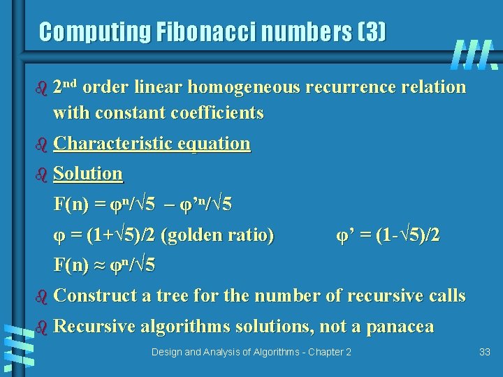
Computing Fibonacci numbers (3) b 2 nd order linear homogeneous recurrence relation with constant coefficients b Characteristic equation b Solution F(n) = φn/√ 5 – φ’n/√ 5 φ = (1+√ 5)/2 (golden ratio) φ’ = (1 -√ 5)/2 F(n) ≈ φn/√ 5 b Construct a tree for the number of recursive calls b Recursive algorithms solutions, not a panacea Design and Analysis of Algorithms - Chapter 2 33

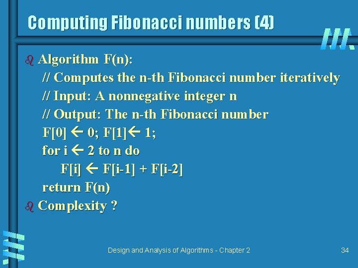
Computing Fibonacci numbers (4) b Algorithm F(n): // Computes the n-th Fibonacci number iteratively // Input: A nonnegative integer n // Output: The n-th Fibonacci number F[0] 0; F[1] 1; for i 2 to n do F[i] F[i-1] + F[i-2] return F(n) b Complexity ? Design and Analysis of Algorithms - Chapter 2 34

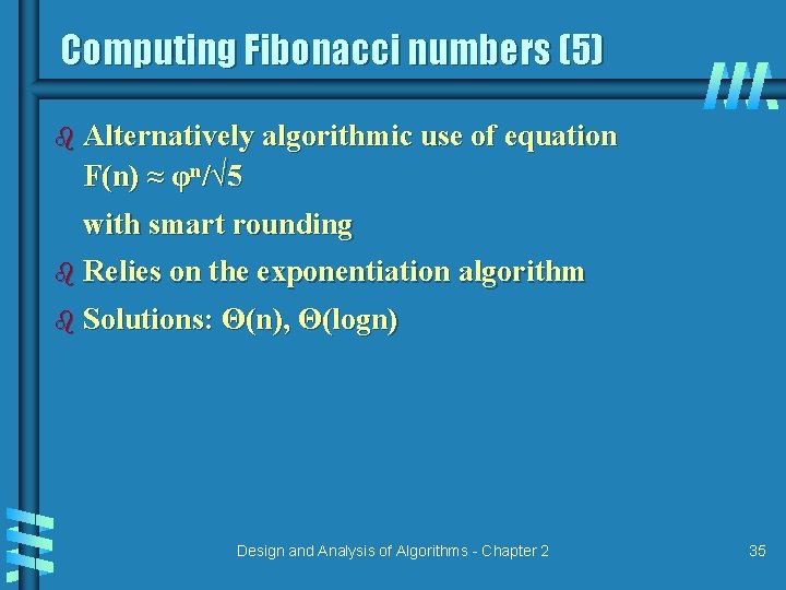
Computing Fibonacci numbers (5) b Alternatively algorithmic use of equation F(n) ≈ φn/√ 5 with smart rounding b Relies on the exponentiation algorithm b Solutions: Θ(n), Θ(logn) Design and Analysis of Algorithms - Chapter 2 35

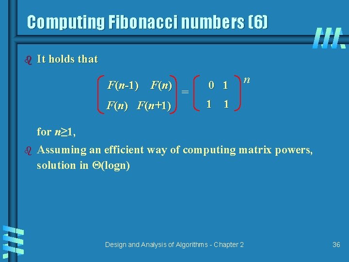
Computing Fibonacci numbers (6) b It holds that F(n-1) F(n) F(n+1) = 0 1 n 1 1 for n≥ 1, b Assuming an efficient way of computing matrix powers, solution in Θ(logn) Design and Analysis of Algorithms - Chapter 2 36

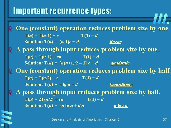
Important recurrence types: b One (constant) operation reduces problem size by one. T(n) = T(n-1) + c T(1) = d Solution: T(n) = (n-1)c + d b A pass through input reduces problem size by one. T(n) = T(n-1) + cn T(1) = d Solution: T(n) = [n(n+1)/2 – 1] c + d b quadratic One (constant) operation reduces problem size by half. T(n) = T(n/2) + c T(1) = d Solution: T(n) = c lg n + d b linear logarithmic A pass through input reduces problem size by half. T(n) = 2 T(n/2) + cn T(1) = d Solution: T(n) = cn lg n + d n n log n Design and Analysis of Algorithms - Chapter 2 37

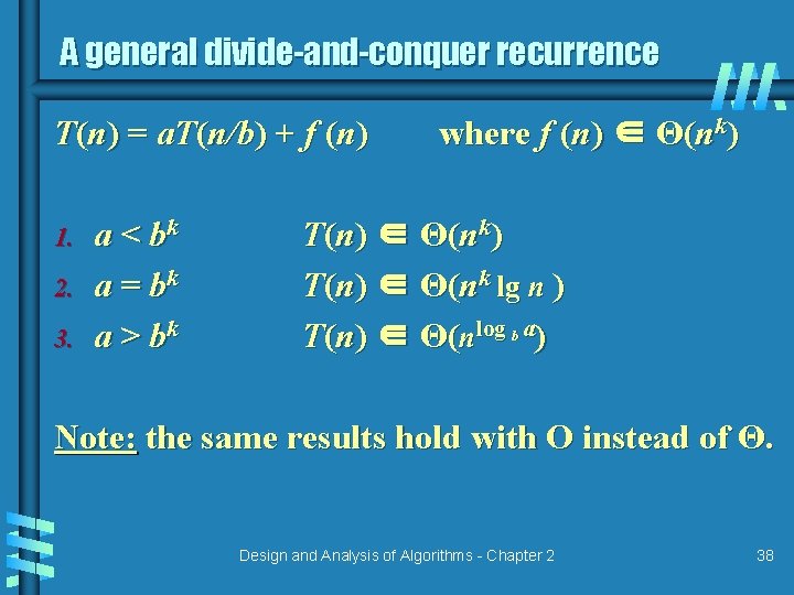
A general divide-and-conquer recurrence T(n) = a. T(n/b) + f (n) 1. 2. 3. a < bk a = bk a > bk where f (n) ∈ Θ(nk) T(n) ∈ Θ(nk lg n ) T(n) ∈ Θ(nlog b a) Note: the same results hold with O instead of Θ. Design and Analysis of Algorithms - Chapter 2 38

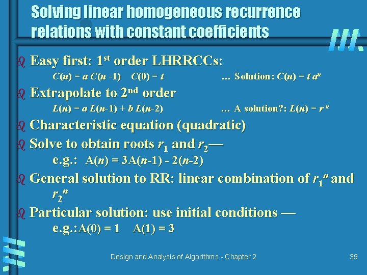
Solving linear homogeneous recurrence relations with constant coefficients b Easy first: 1 st order LHRRCCs: C(n) = a C(n -1) C(0) = t … Solution: C(n) = t an b Extrapolate to 2 nd order L(n) = a L(n-1) + b L(n-2) … A solution? : L(n) = r n b Characteristic equation (quadratic) b Solve to obtain roots r 1 and r 2— e. g. : A(n) = 3 A(n-1) - 2(n-2) b General solution to RR: linear combination of r 1 n and r 2 n b Particular solution: use initial conditions — e. g. : A(0) = 1 A(1) = 3 Design and Analysis of Algorithms - Chapter 2 39