Analysis and propagation of errors Peter Fox GIS

Analysis and propagation of errors Peter Fox GIS for Science ERTH 4750 (98271) Week 8, Tuesday, March 20, 2012 1

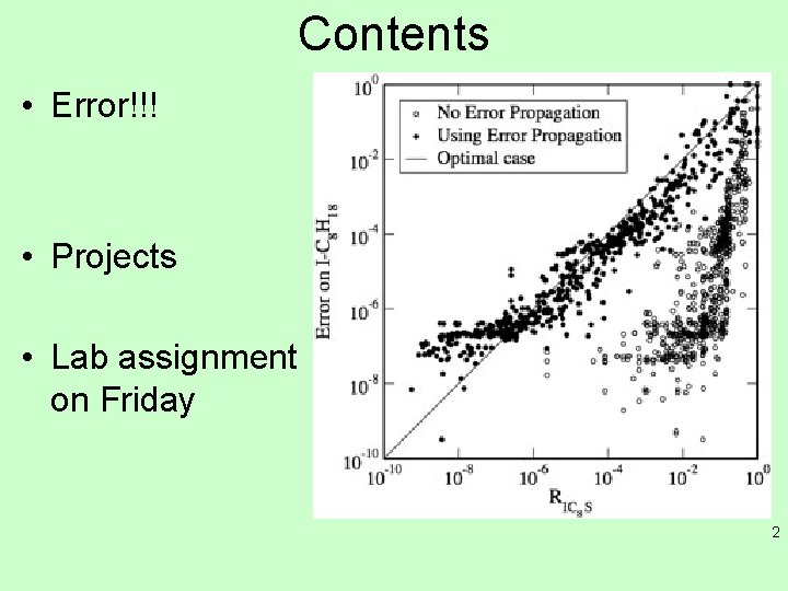
Contents • Error!!! • Projects • Lab assignment on Friday 2

Spatial analysis of continuous fields • Possibly more important than our answer is our confidence in the answer. • Our confidence is quantified by uncertainties as discussed earlier. • Once we combine numbers, we need to be able to assess how the uncertainties change for the combination. • This is called propagation of errors or more correctly the propagation of our understanding/ estimate of errors in the result we are looking at… 3

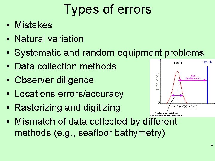
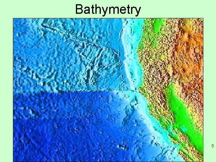
Types of errors • • Mistakes Natural variation Systematic and random equipment problems Data collection methods Observer diligence Locations errors/accuracy Rasterizing and digitizing Mismatch of data collected by different methods (e. g. , seafloor bathymetry) 4

Bathymetry 5

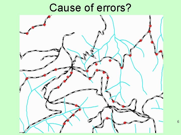
Cause of errors? 6

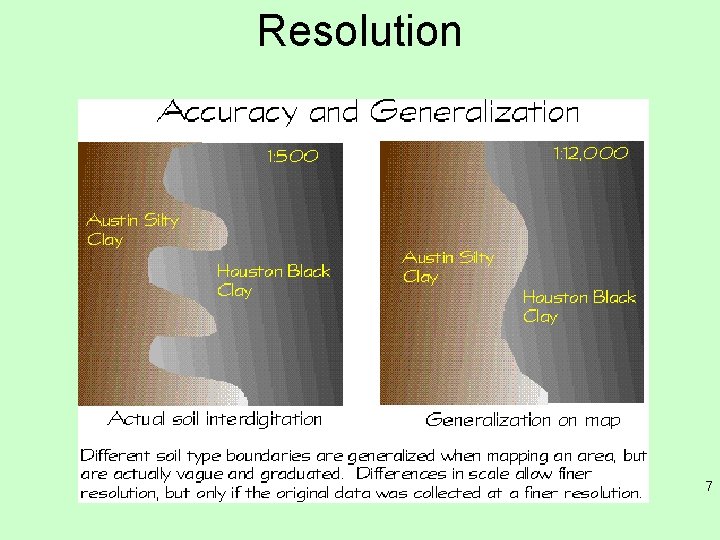
Resolution 7

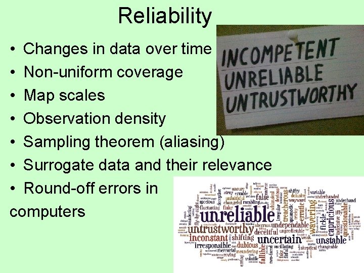
Reliability • Changes in data over time • Non-uniform coverage • Map scales • Observation density • Sampling theorem (aliasing) • Surrogate data and their relevance • Round-off errors in computers 8

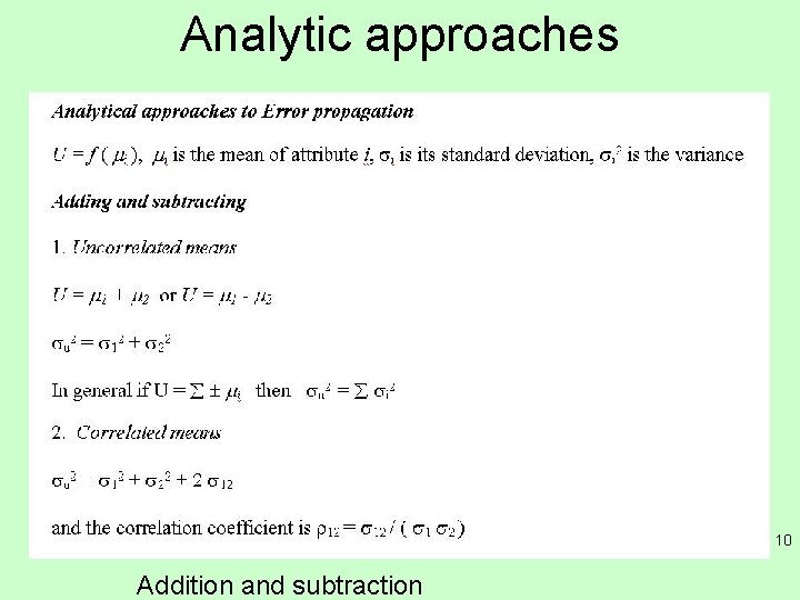
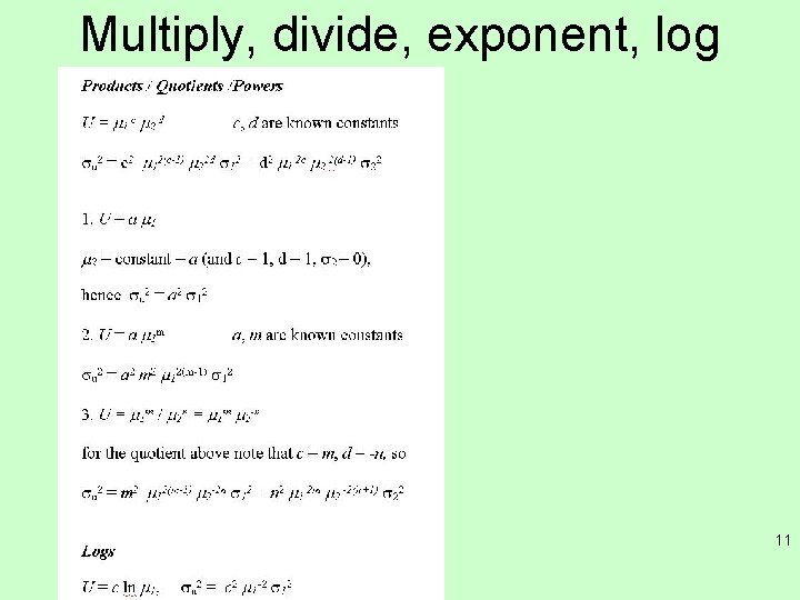
Error propagation • Errors arise from data quality, model quality and data/model interaction. • We need to know the sources of the errors and how they propagate through our model. • Simplest representation of errors is to treat observations/attributes as statistical data – use mean and standard deviation. 9

Analytic approaches 10 Addition and subtraction

Multiply, divide, exponent, log 11

Monte Carlo simulation • If a new attribute U is given by U = f (A 1, A 2, A 3, …. An) where the A’s are attributes and f represents some function combining them, then we want to know what is the standard deviation of the combination U and how does the standard deviation of each A contribute to it? • By MC simulation we look at the statistical distribution of a lot of realizations (random samples) of U. 12

MC (ctd) • A single realization of U is Ui = f (R 1, R 2, R 3, …. Rn) where each Rn is a random sample of its corresponding attribute An based on the statistical properties (mean and standard deviation, for example) of An. • The probability functions for the attributes themselves need not be Gaussian and could even be taken from histograms of observed values. 13

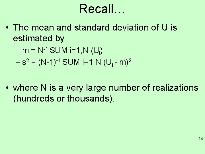
Recall… • The mean and standard deviation of U is estimated by – m = N-1 SUM i=1, N (Ui) – s 2 = (N-1)-1 SUM i=1, N (Ui - m)2 • where N is a very large number of realizations (hundreds or thousands). 14

When to use? • MC simulation is most useful when the function relating the attributes is complex or the statistical distribution is known only empirically (from a histogram, for example). • For simpler combinations of attributes, there are easier, direct (analytical) ways to estimate the new uncertainties from the attribute uncertainties. 15

Generating pseudo random numbers • For the Monte Carlo simulation, you will want to generate a series of random numbers with a normal (bell-curve) distribution. • There are 2 ways to do this in Excel. • In older versions of Excel, you can use the Tools > Data Analysis > Random number generation > Normal distribution to generate a sequence of random numbers. 16

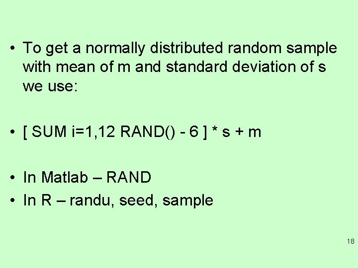
Second way • Or, you can take advantage of the central limit theorem that states that under certain conditions, random samples of any distribution will have a normal distribution. • The Excel function RAND generates a uniformly distributed random number, that is, the probability is the same for any number between 0 and 1 to be generated. • To get a normally distributed random sample with mean of 0 and standard deviation of 1 we can simply add 12 uniformly distributed random numbers and subtract 6. 17

• To get a normally distributed random sample with mean of m and standard deviation of s we use: • [ SUM i=1, 12 RAND() - 6 ] * s + m • In Matlab – RAND • In R – randu, seed, sample 18

Tip • Because this expression is quite long in Excel you can create a macro to facilitate using it again and again. • To record a macro, select Tools > Macro > Record new macro > give name to the macro > ok > type in expression > Stop recording. • You can refer to re-named cells from within a macro, so you might want to use variable names for the mean and standard deviation to keep your macro general. 19

Shortcuts • You can also specify a Control-key to run the macro from the worksheet. Otherwise, to run the macro, go to Tools > Macros > select the macro name and press Run. • Once the macro is run in a cell, you can drag the expression to other cells using the drag handle in the lower-right corner of the cell. 20

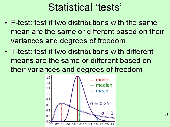
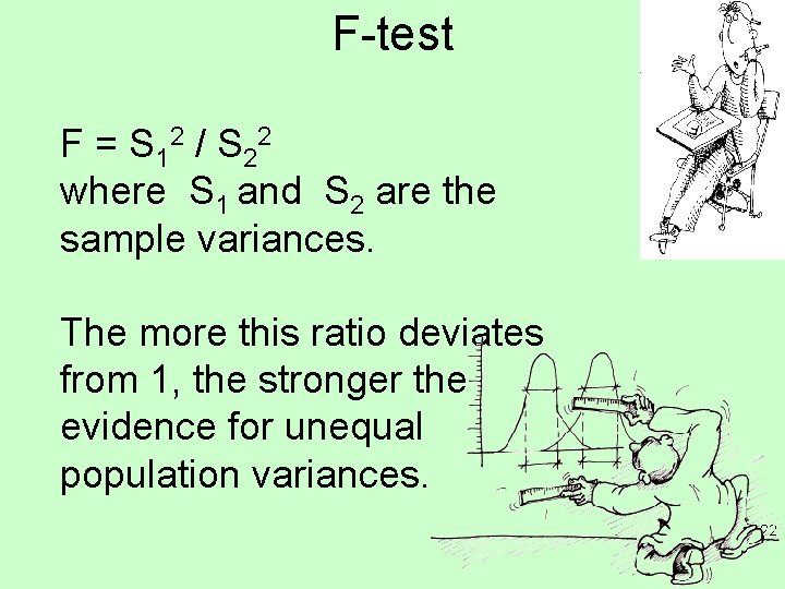
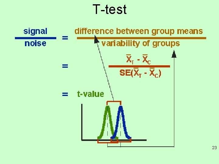
Statistical ‘tests’ • F-test: test if two distributions with the same mean are the same or different based on their variances and degrees of freedom. • T-test: test if two distributions with different means are the same or different based on their variances and degrees of freedom 21

F-test F = S 12 / S 22 where S 1 and S 2 are the sample variances. The more this ratio deviates from 1, the stronger the evidence for unequal population variances. 22

T-test 23

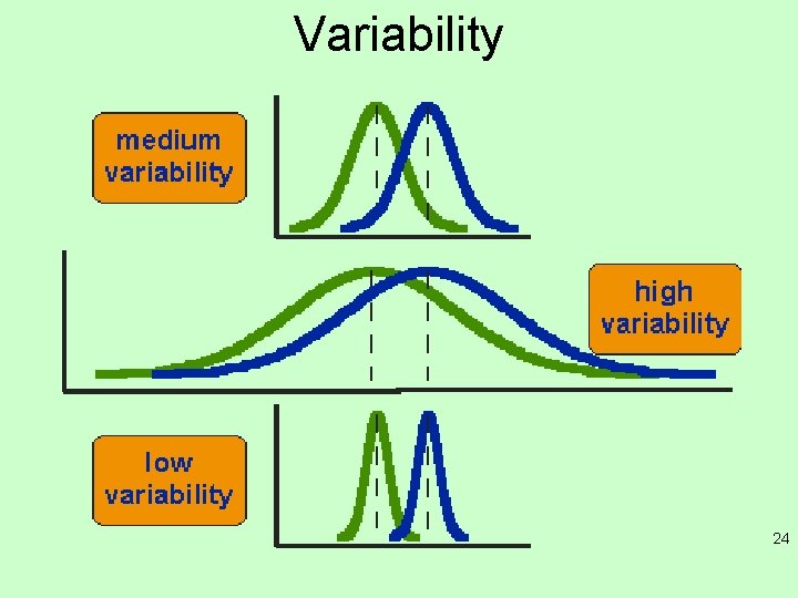
Variability 24

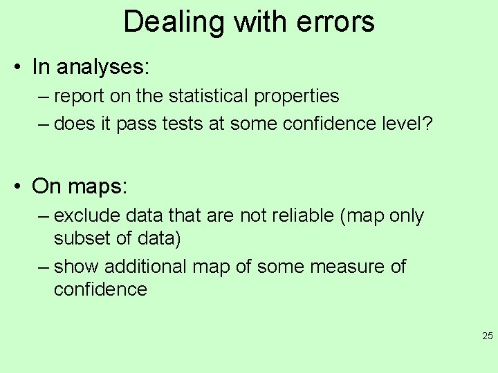
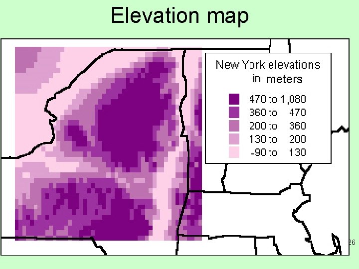
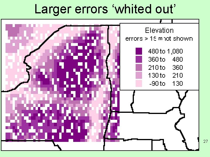
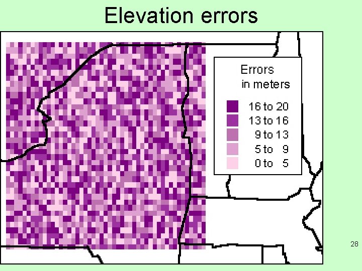
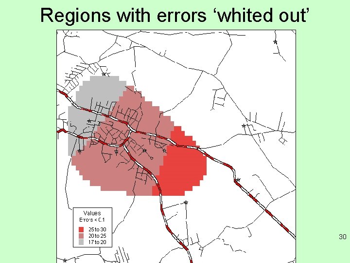
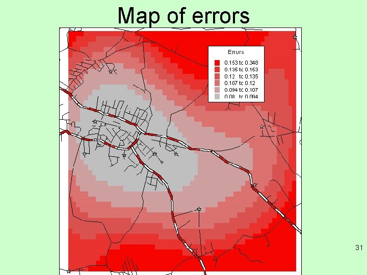
Dealing with errors • In analyses: – report on the statistical properties – does it pass tests at some confidence level? • On maps: – exclude data that are not reliable (map only subset of data) – show additional map of some measure of confidence 25

Elevation map meters 26

Larger errors ‘whited out’ m 27

Elevation errors meters 28

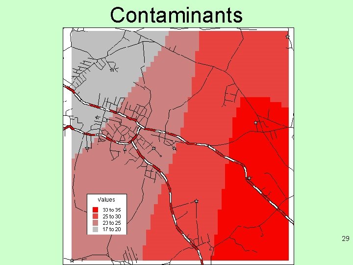
Contaminants 29

Regions with errors ‘whited out’ 30

Map of errors 31

Summary • Topics for GIS (for Science) – Estimating, propagating and displaying error considerations • For learning purposes remember: – Demonstrate proficiency in using geospatial applications and tools (commercial and open-source). – Present verbally relational analysis and interpretation of a variety of spatial data on maps. – Demonstrate skill in applying database concepts to build and manipulate a spatial database, SQL, spatial queries, and integration of graphic and tabular data. – Demonstrate intermediate knowledge of geospatial analysis methods and their applications. 32

Friday Mar. 23 • Lab assignment session – three problems, up on ~ Wednesday • Complete them in class, get signed off before leaving • 10% of grade 33

Reading for this week • http: //www. chemtopics. com/aplab/errors. pdf • http: //www. nuim. ie/staff/dpringle/gis 11. pdf 34

Next classes • Friday, March 23 – lab with material from week 7 (lab assignment 10%) • Tuesday, March 27, Using uncertainties, working with discrete entity types • Note March 30 – open lab (no assignment, work on your projects, get help from Max), attendance will be taken 35