Analyses of Variance Simple Situation Genotype A 135

Analyses of Variance

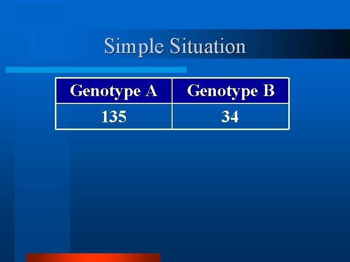
Simple Situation Genotype A 135 Genotype B 34

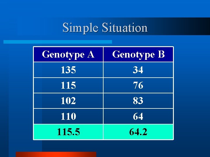
Simple Situation Genotype A 135 115 102 110 115. 5 Genotype B 34 76 83 64 64. 2

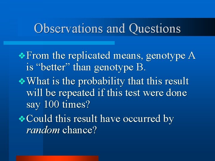
Observations and Questions v From the replicated means, genotype A is “better” than genotype B. v What is the probability that this result will be repeated if this test were done say 100 times? v Could this result have occurred by random chance?

t-test |x 1 -x 2| t= 2[( 12+ 22)/(n 1+n 2)]

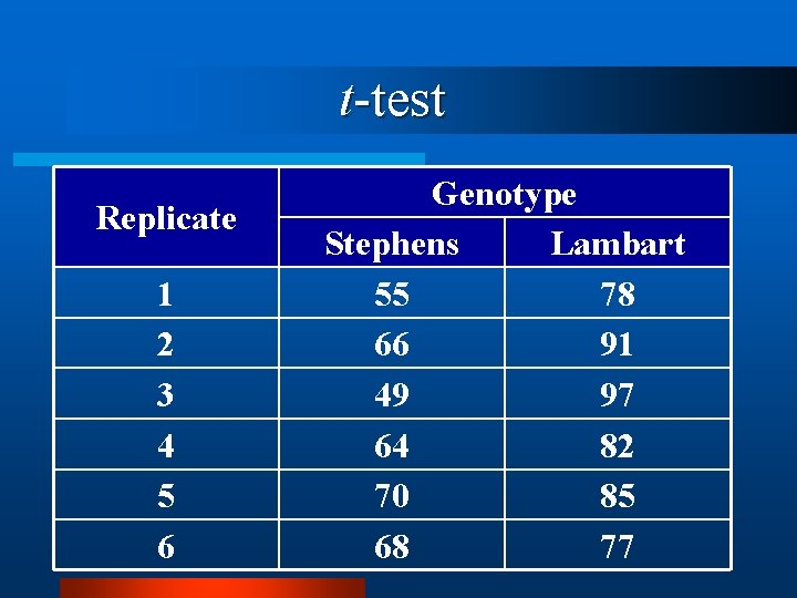
t-test Replicate 1 2 3 4 5 6 Genotype Stephens Lambart 55 78 66 91 49 97 64 82 70 85 68 77

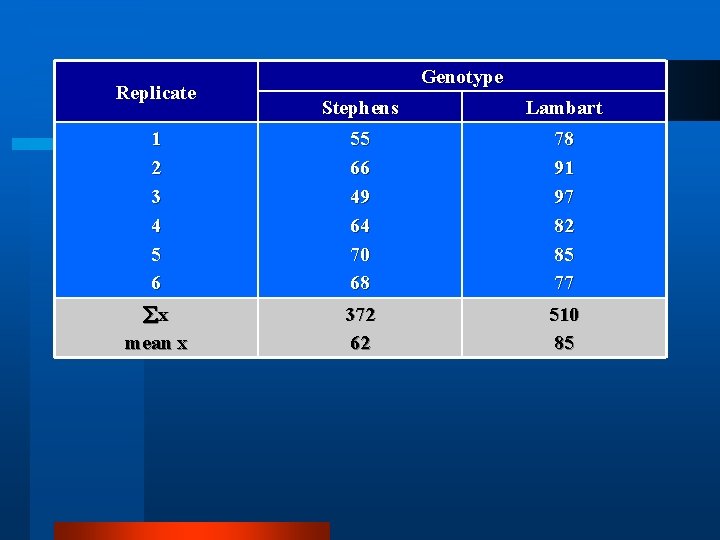
Replicate Genotype Stephens Lambart 1 2 3 4 5 6 55 66 49 64 70 68 78 91 97 82 85 77 x mean x 372 62 510 85

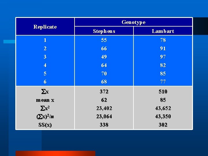
Replicate Genotype Stephens Lambart 1 2 3 4 5 6 55 66 49 64 70 68 78 91 97 82 85 77 x mean x x 2 ( x)2/n SS(x) 372 62 23, 402 23, 064 338 510 85 43, 652 43, 350 302

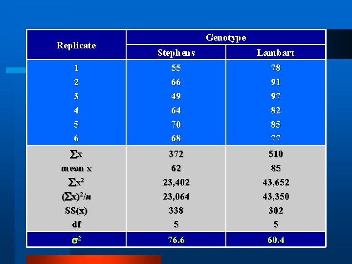
Replicate Genotype Stephens Lambart 1 2 3 4 5 6 55 66 49 64 70 68 78 91 97 82 85 77 x mean x x 2 ( x)2/n SS(x) df 372 62 23, 402 23, 064 338 5 510 85 43, 652 43, 350 302 5 2 76. 6 60. 4

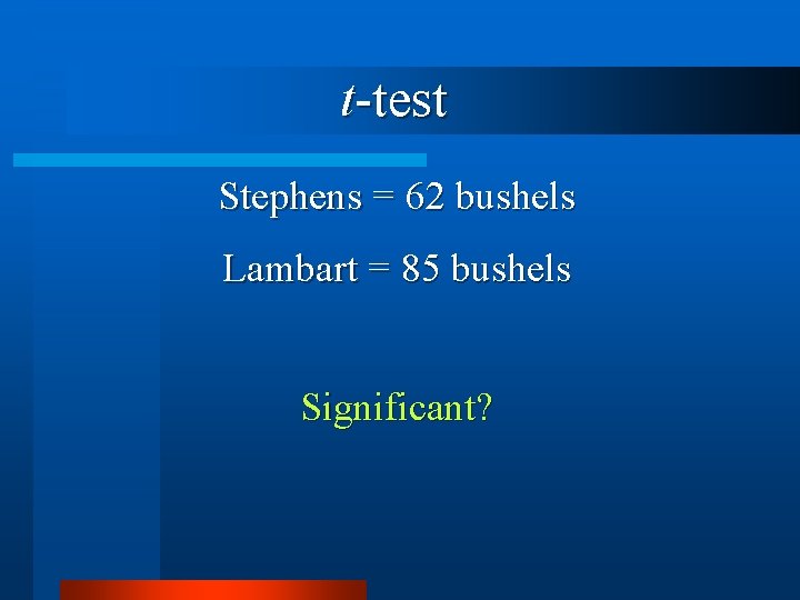
t-test Stephens = 62 bushels Lambart = 85 bushels Significant?

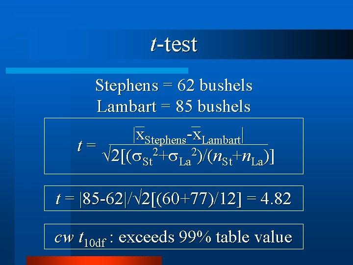
t-test Stephens = 62 bushels Lambart = 85 bushels |x. Stephens-x. Lambart| t= 2[( St 2+ La 2)/(n. St+n. La)] t = |85 -62|/ 2[(60+77)/12] = 4. 82 cw t 10 df : exceeds 99% table value

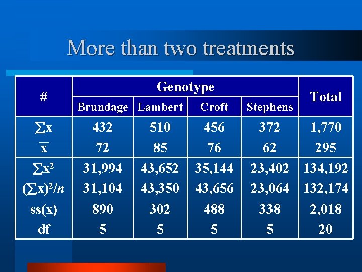
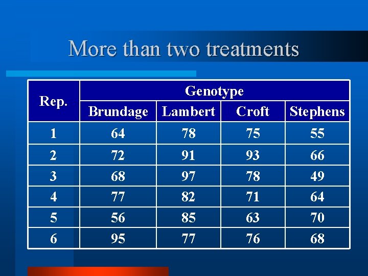
More than two treatments Rep. Genotype Brundage Lambert Croft Stephens 1 64 78 75 55 2 3 4 5 6 72 68 77 56 95 91 97 82 85 77 93 78 71 63 76 66 49 64 70 68

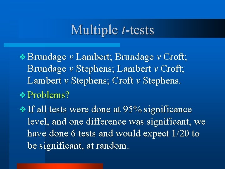
Multiple t-tests v Brundage v Lambert; Brundage v Croft; Brundage v Stephens; Lambert v Croft; Lambert v Stephens; Croft v Stephens. v Problems? v If all tests were done at 95% significance level, and one difference was significant, we have done 6 tests and would expect 1/20 to be significant, at random.

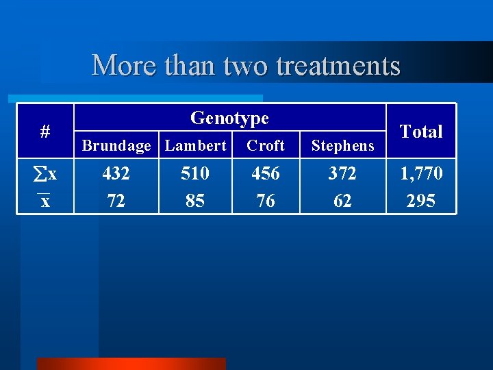
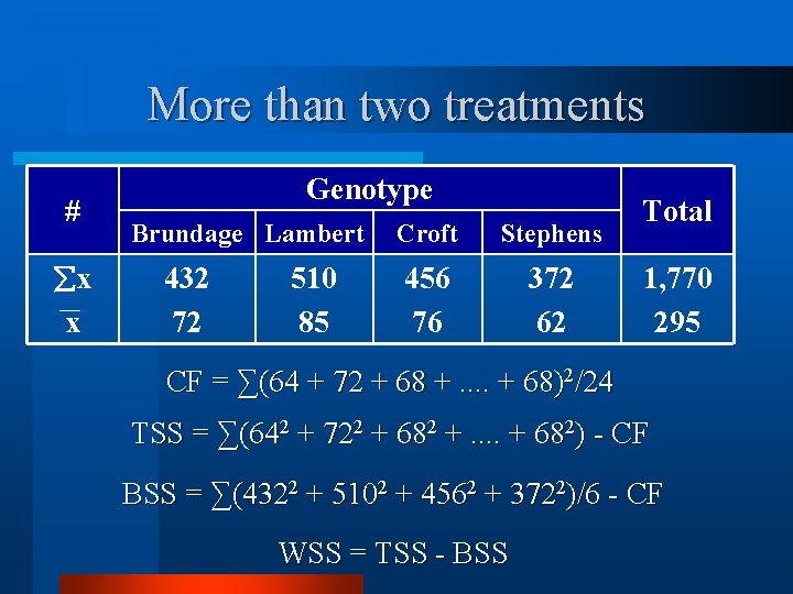
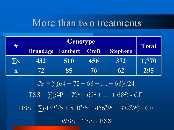
More than two treatments # x x Genotype Brundage Lambert 432 72 510 85 Croft Stephens 456 76 372 62 Total 1, 770 295

More than two treatments # x x x 2 ( x)2/n ss(x) df Genotype Brundage Lambert 432 72 31, 994 31, 104 890 5 510 85 43, 652 43, 350 302 5 Croft 456 76 35, 144 43, 656 488 5 Stephens Total 372 1, 770 62 295 23, 402 134, 192 23, 064 132, 174 338 2, 018 5 20

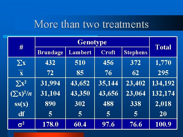
More than two treatments # x x x 2 ( x)2/n ss(x) df 2 Genotype Brundage Lambert 432 72 31, 994 31, 104 890 5 178. 0 510 85 43, 652 43, 350 302 5 60. 4 Croft 456 76 35, 144 43, 656 488 5 97. 6 Stephens Total 372 1, 770 62 295 23, 402 134, 192 23, 064 132, 174 338 2, 018 5 20 76. 6 100. 9

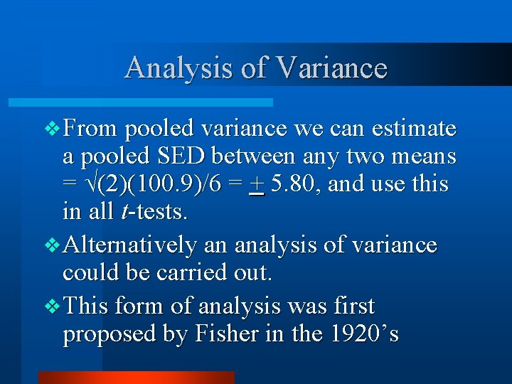
Analysis of Variance v From pooled variance we can estimate a pooled SED between any two means = (2)(100. 9)/6 = + 5. 80, and use this in all t-tests. v Alternatively an analysis of variance could be carried out. v This form of analysis was first proposed by Fisher in the 1920’s

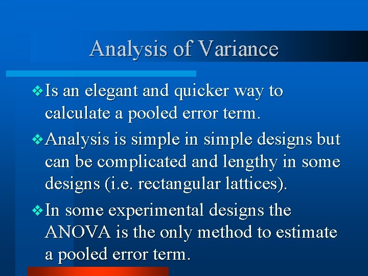
Analysis of Variance v Is an elegant and quicker way to calculate a pooled error term. v Analysis is simple in simple designs but can be complicated and lengthy in some designs (i. e. rectangular lattices). v In some experimental designs the ANOVA is the only method to estimate a pooled error term.

Analysis of Variance v It can provide an F-test to tests specific hypotheses. (i. e. to test general differences between different treatments). v Can be an invaluable initial contribution to interpretation of experiments.

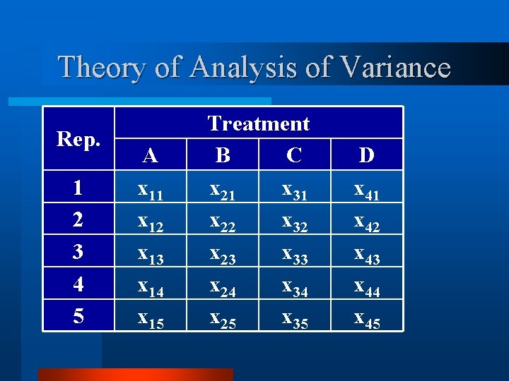
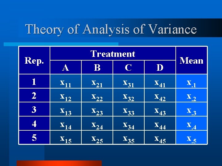
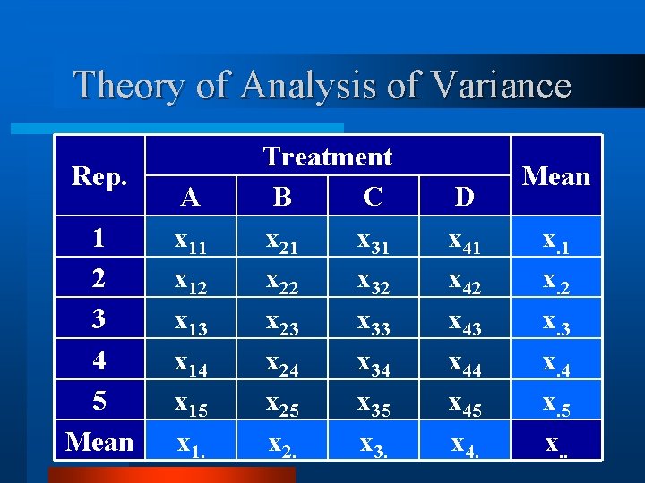
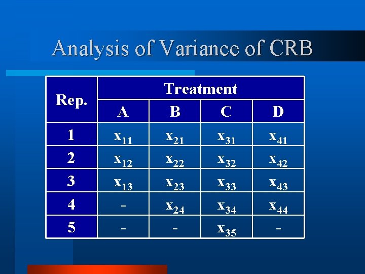
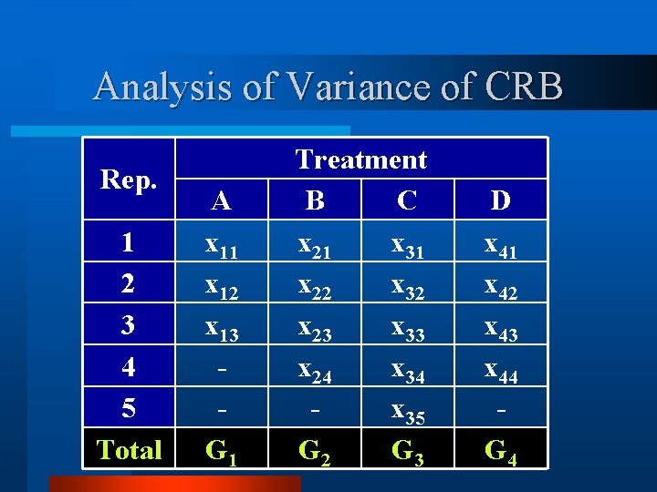
Theory of Analysis of Variance v Consider a simple CRB design. v Four treatments (n = 4). v With all treatments replicated 5 times (k = 5). v The total experiment would be n x k = 20 experimental units.

Theory of Analysis of Variance Rep. 1 2 3 4 5 A x 11 x 12 x 13 x 14 x 15 Treatment B C x 21 x 31 x 22 x 32 x 23 x 33 x 24 x 34 x 25 x 35 D x 41 x 42 x 43 x 44 x 45

Theory of Analysis of Variance Rep. 1 2 3 4 5 A x 11 x 12 x 13 x 14 x 15 Treatment B C x 21 x 31 x 22 x 32 x 23 x 33 x 24 x 34 x 25 x 35 D x 41 x 42 x 43 x 44 x 45 Mean x. 1 x. 2 x. 3 x. 4 x. 5

Theory of Analysis of Variance Rep. 1 2 3 4 5 Mean A x 11 x 12 x 13 x 14 x 15 x 1. Treatment B C x 21 x 31 x 22 x 32 x 23 x 33 x 24 x 34 x 25 x 35 x 2. x 3. D x 41 x 42 x 43 x 44 x 45 x 4. Mean x. 1 x. 2 x. 3 x. 4 x. 5 x. .

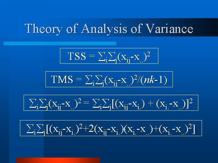
Theory of Analysis of Variance TSS = i j(xij-x. . )2 TMS = i j(xij-x. . )2/(nk-1) i j(xij-x. . )2 = i j[(xij-xi. ) + (xi. -x. . )]2 i j[(xij-xi. )2+2(xij-xi. )(xi. -x. . )+(xi. -x. . )2]

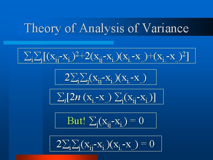
Theory of Analysis of Variance i j[(xij-xi. )2+2(xij-xi. )(xi. -x. . )+(xi. -x. . )2] 2 i j(xij-xi. )(xi. -x. . ) i[2 n (xi. -x. . ) j(xij-xi. )] But! j(xij-xi. ) = 0 2 i j(xij-xi. )(xi. -x. . ) = 0

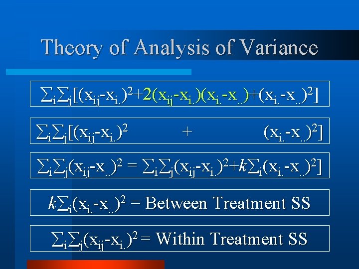
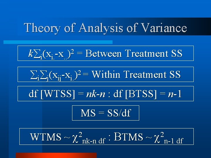
Theory of Analysis of Variance i j[(xij-xi. )2+2(xij-xi. )(xi. -x. . )+(xi. -x. . )2] i j[(xij-xi. )2 + (xi. -x. . )2] i j(xij-x. . )2 = i j(xij-xi. )2+k i(xi. -x. . )2] k i(xi. -x. . )2 = Between Treatment SS i j(xij-xi. )2 = Within Treatment SS

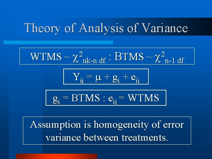
Theory of Analysis of Variance k i(xi. -x. . )2 = Between Treatment SS i j(xij-xi. )2 = Within Treatment SS df [WTSS] = nk-n : df [BTSS] = n-1 MS = SS/df WTMS ~ 2 nk-n df : BTMS ~ 2 n-1 df

Theory of Analysis of Variance WTMS ~ 2 nk-n df : BTMS ~ 2 n-1 df Yij = + gi + eij gi = BTMS : eij = WTMS Assumption is homogeneity of error variance between treatments.

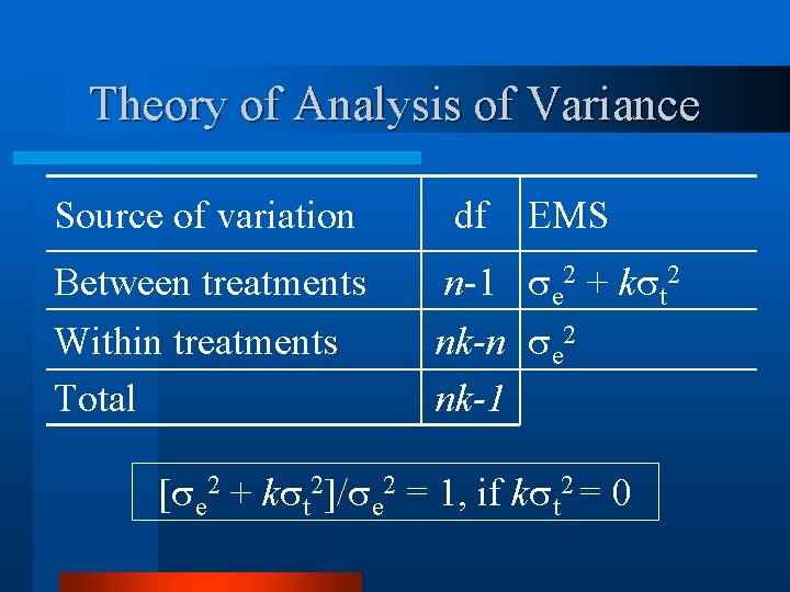
Theory of Analysis of Variance Source of variation df EMS Between treatments n-1 e 2 + k t 2 Within treatments Total nk-n e 2 nk-1 [ e 2 + k t 2]/ e 2 = 1, if k t 2 = 0

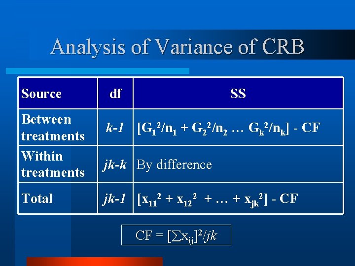
Analysis of Variance of CRB Source Between treatments Within treatments Total df SS k-1 [G 12/n 1 + G 22/n 2 … Gk 2/nk] - CF jk-k By difference jk-1 [x 112 + x 122 + … + xjk 2] - CF CF = [ xij]2/jk

More than two treatments Rep. Genotype Brundage Lambert Croft Stephens 1 64 78 75 55 2 3 4 5 6 72 68 77 56 95 91 97 82 85 77 93 78 71 63 76 66 49 64 70 68

More than two treatments Genotype # Brundage Lambert x x 432 72 510 85 Croft Stephens 456 76 372 62 Total 1, 770 295 CF = ∑(64 + 72 + 68 +. . + 68)2/24 TSS = ∑(642 + 722 + 682 +. . + 682) - CF BSS = ∑(4322/6 + 5102/6 + 4562/6 + 3722/6) - CF WSS = TSS - BSS

More than two treatments # x x Genotype Brundage Lambert 432 72 510 85 Croft Stephens 456 76 372 62 Total 1, 770 295 CF = ∑(64 + 72 + 68 +. . + 68)2/24 TSS = ∑(642 + 722 + 682 +. . + 682) - CF BSS = ∑(4322 + 5102 + 4562 + 3722)/6 - CF WSS = TSS - BSS

More than two treatments Genotype # Brundage Lambert x x 432 72 510 85 Croft Stephens 456 76 372 62 Total 1, 770 295 CF = ∑(64 + 72 + 68 +. . + 68)2/24 TSS = ∑(642 + 722 + 682 +. . + 682) - CF BSS = ∑(4322/6 + 5102/6 + 4562/6 + 3722/6) - CF WSS = TSS - BSS

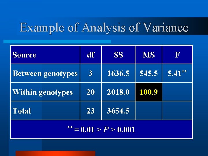
Example of Analysis of Variance Source df SS MS F Between genotypes 3 1636. 5 545. 5 5. 41** Within genotypes 20 2018. 0 100. 9 Total 23 3654. 5 ** = 0. 01 > P > 0. 001

Analysis of Variance of CRB Rep. 1 2 3 4 5 A x 11 x 12 x 13 - Treatment B C x 21 x 31 x 22 x 32 x 23 x 33 x 24 x 35 D x 41 x 42 x 43 x 44 -

Analysis of Variance of CRB Rep. 1 2 3 4 5 Total A x 11 x 12 x 13 G 1 Treatment B C x 21 x 31 x 22 x 32 x 23 x 33 x 24 x 35 G 2 G 3 D x 41 x 42 x 43 x 44 G 4

Analysis of Variance of CRB Rep. 1 2 3 4 5 Total A x 11 x 12 x 13 G 1 Treatment B C x 21 x 31 x 22 x 32 x 23 x 33 x 24 x 35 G 2 G 3 D x 41 x 42 x 43 x 44 G 4

Analysis of Variance of CRB Source Between treatments Within treatments Total df SS k-1 [G 12/n 1 + G 22/n 2 … Gk 2/nk] - CF jk-k By difference jk-1 [x 112 + x 122 + … + xjk 2] - CF CF = [ xij]2/jk

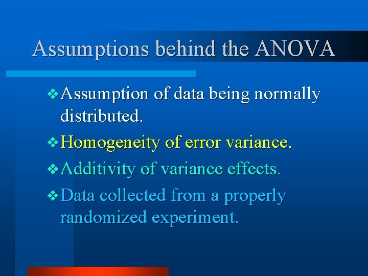
Assumptions behind the ANOVA v Assumption of data being normally distributed. v Homogeneity of error variance. v Additivity of variance effects. v Data collected from a properly randomized experiment.

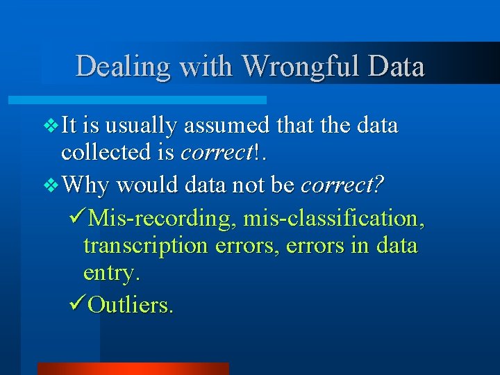
Dealing with Wrongful Data v It is usually assumed that the data collected is correct!. v Why would data not be correct? üMis-recording, mis-classification, transcription errors, errors in data entry. üOutliers.

Dealing with Wrongful Data v What things can help? üKeep detailed records, on each experimental unit. üDecide beforehand what values would arouse suspision.

Dealing with Wrongful Data v What do you do with suspicios data? üIf correct, and it is discarded, then valuable information is lost. This will bias the results. üIf wrong and included, will bias results and may have extreme consequences.

Checking ANOVA Accurucy v Coefficient of variation: [ e/ ]x 100. v CV=(√ 100. 9/73. 75)*100=13. 6% v. R 2 value = {[TSS-ESS]/TSS}x 100. v. R 2 = (1654/3654)*100 = 44. 7%. v. Compare the effect of blocking or sub-blocking (discussed later).

Next Class ANOVA of RCB Designs ANOVA of Latin Square Designs