Analyses of Variance Assumptions behind the ANOVA v

Analyses of Variance

Assumptions behind the ANOVA v Assumption of data being normally distributed. v Homogeneity of error variance. v Additivity of variance effects. v Data collected from a properly randomized experiment.

Dealing with Wrongful Data v It is usually assumed that the data collected is correct!. v Why would data not be correct? üMis-recording, mis-classification, transcription errors, errors in data entry. üOutliers.
Dealing with Wrongful Data v What things can help? üKeep detailed records, on each experimental unit. üDecide beforehand what values would arouse suspision.

Dealing with Wrongful Data v What do you do with suspicios data? üIf correct, and it is discarded, then valuable information is lost. This will bias the results. üIf wrong and included, will bias results and may have extreme consequences.
![Checking ANOVA Accurucy v Coefficient of variation: [ e/ ]x 100. v CV=(√ 100. Checking ANOVA Accurucy v Coefficient of variation: [ e/ ]x 100. v CV=(√ 100.](http://slidetodoc.com/presentation_image_h2/3ec68cfa5208881f20fdb70624c8c654/image-6.jpg)
Checking ANOVA Accurucy v Coefficient of variation: [ e/ ]x 100. v CV=(√ 100. 9/73. 75)*100=13. 6% v. R 2 value = {[TSS-ESS]/TSS}x 100. v. R 2 = (1654/3654)*100 = 44. 7%. v. Compare the effect of blocking or sub-blocking (discussed later).

Analyses of CRB Designs Yij = + ti eij

Analysis of Variance of CRB Source Between treatments Within treatments Total df SS k-1 [G 12/n 1 + G 22/n 2 … Gk 2/nk] - CF jk-k By difference jk-1 [x 112 + x 122 + … + xjk 2] - CF CF = [ xij]2/jk
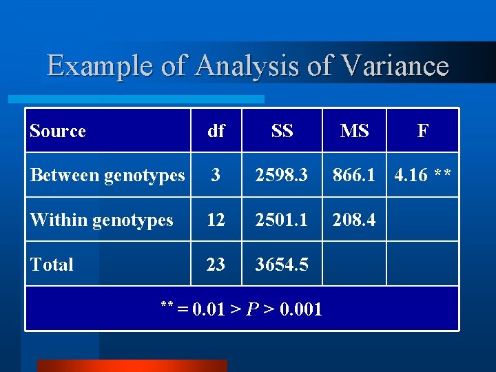
Example of Analysis of Variance Source df SS Between genotypes 3 2598. 3 866. 1 4. 16 ** Within genotypes 12 2501. 1 208. 4 Total 23 3654. 5 ** = 0. 01 > P > 0. 001 MS F

Analyses of RCB Designs Yij = + bi + tj + eij
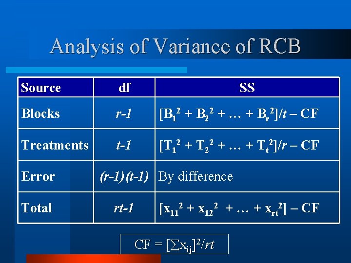
Analysis of Variance of RCB Source df Blocks r-1 [B 12 + B 22 + … + Br 2]/t – CF Treatments t-1 [T 12 + T 22 + … + Tt 2]/r – CF Error Total SS (r-1)(t-1) By difference rt-1 [x 112 + x 122 + … + xrt 2] – CF CF = [ xij]2/rt
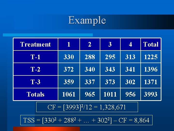
Example Treatment 1 2 3 4 Total T-1 330 288 295 313 1225 T-2 372 340 343 341 1396 T-3 359 337 373 302 1371 Totals 1061 965 1011 956 3993 CF = [3993]2/12 = 1, 328, 671 TSS = [3302 + 2882 + … + 3022] – CF = 8, 864
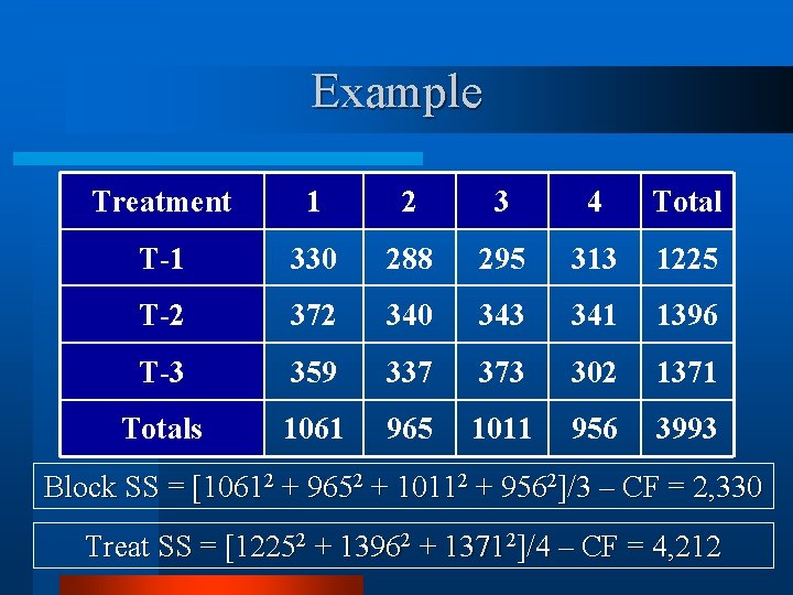
Example Treatment 1 2 3 4 Total T-1 330 288 295 313 1225 T-2 372 340 343 341 1396 T-3 359 337 373 302 1371 Totals 1061 965 1011 956 3993 Block SS = [10612 + 9652 + 10112 + 9562]/3 – CF = 2, 330 Treat SS = [12252 + 13962 + 13712]/4 – CF = 4, 212
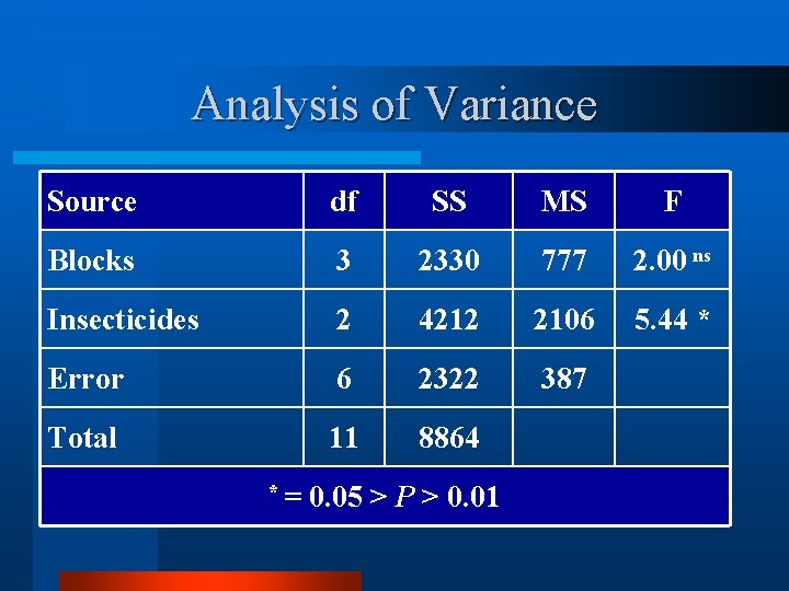
Analysis of Variance Source df SS MS F Blocks 3 2330 777 2. 00 ns Insecticides 2 4212 2106 5. 44 * Error 6 2322 387 Total 11 8864 *= 0. 05 > P > 0. 01
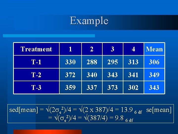
Example Treatment 1 2 3 4 Mean T-1 330 288 295 313 306 T-2 372 340 343 341 349 T-3 359 337 373 302 343 sed[mean] = (2 e 2)/4 = (2 x 387)/4 = 13. 9 6 df se[mean] = ( e 2)/4 = (387/4) = 9. 8 6 df

Analyses of Latin Designs Yijk = + ri + cj + tk(ij) + eijk
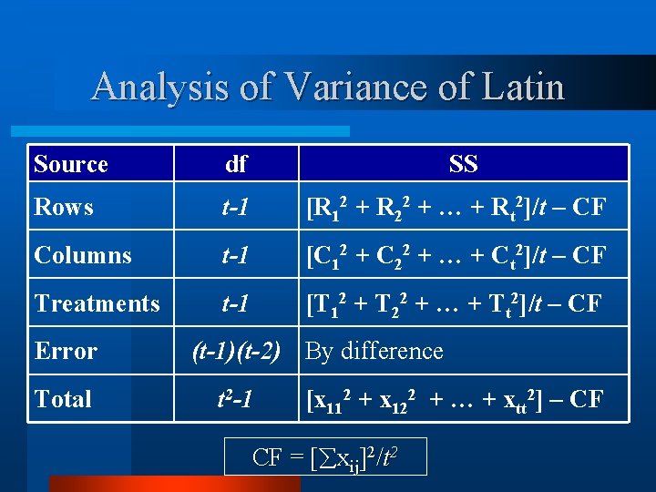
Analysis of Variance of Latin Source df Rows t-1 [R 12 + R 22 + … + Rt 2]/t – CF Columns t-1 [C 12 + C 22 + … + Ct 2]/t – CF Treatments t-1 [T 12 + T 22 + … + Tt 2]/t – CF Error Total SS (t-1)(t-2) By difference t 2 -1 [x 112 + x 122 + … + xtt 2] – CF CF = [ xij]2/t 2
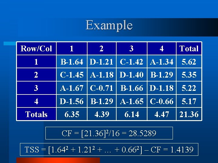
Example Row/Col 1 2 3 4 Total 1 B-1. 64 D-1. 21 C-1. 42 A-1. 34 5. 62 2 C-1. 45 A-1. 18 D-1. 40 B-1. 29 5. 35 3 A-1. 67 C-0. 71 B-1. 66 D-1. 18 5. 22 4 D-1. 56 B-1. 29 A-1. 65 C-0. 66 5. 17 Totals 6. 35 4. 39 6. 14 4. 47 21. 36 CF = [21. 36]2/16 = 28. 5289 TSS = [1. 642 + 1. 212 + … + 0. 662] – CF = 1. 4139

Example Row/Col 1 2 3 4 Total 1 B-1. 64 D-1. 21 C-1. 42 A-1. 34 5. 62 2 C-1. 45 A-1. 18 D-1. 40 B-1. 29 5. 35 3 A-1. 67 C-0. 71 B-1. 66 D-1. 18 5. 22 4 D-1. 56 B-1. 29 A-1. 65 C-0. 66 5. 17 Totals 6. 35 4. 39 6. 14 4. 47 21. 36 Row SS = [5. 622 + 5. 352 + 5. 222 + 5. 172]/4 – CF = 0. 0301 Col SS = [6. 352 + 4. 392 + 6. 142 + 4. 472]/4 – CF = 0. 8273
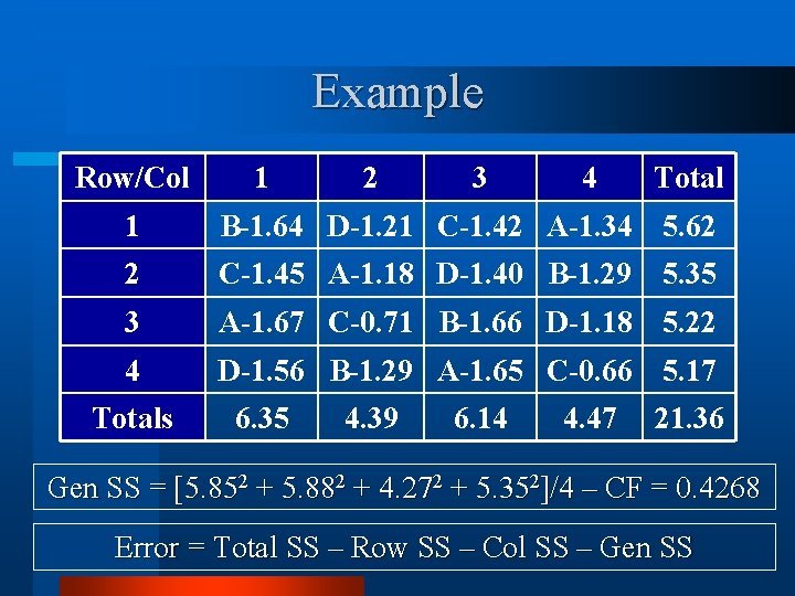
Example Row/Col 1 2 3 4 Total 1 B-1. 64 D-1. 21 C-1. 42 A-1. 34 5. 62 2 C-1. 45 A-1. 18 D-1. 40 B-1. 29 5. 35 3 A-1. 67 C-0. 71 B-1. 66 D-1. 18 5. 22 4 D-1. 56 B-1. 29 A-1. 65 C-0. 66 5. 17 Totals 6. 35 4. 39 6. 14 4. 47 21. 36 Gen SS = [5. 852 + 5. 882 + 4. 272 + 5. 352]/4 – CF = 0. 4268 Error = Total SS – Row SS – Col SS – Gen SS
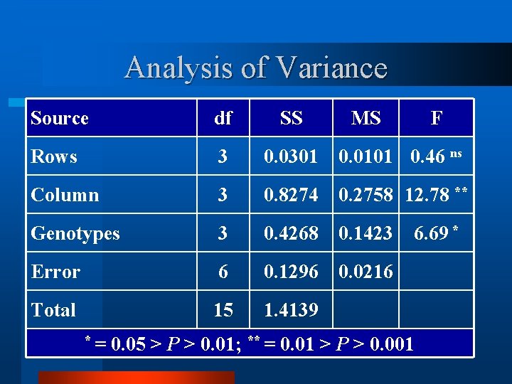
Analysis of Variance Source df SS Rows 3 0. 0301 0. 0101 0. 46 ns Column 3 0. 8274 0. 2758 12. 78 ** Genotypes 3 0. 4268 0. 1423 Error 6 0. 1296 0. 0216 Total 15 1. 4139 *= MS F 6. 69 * 0. 05 > P > 0. 01; ** = 0. 01 > P > 0. 001
![Efficiency of Latin Squares cw CRB Design [MSr + MSc + (t-1)EMS]/(t+1)EMS [0. 0100+0. Efficiency of Latin Squares cw CRB Design [MSr + MSc + (t-1)EMS]/(t+1)EMS [0. 0100+0.](http://slidetodoc.com/presentation_image_h2/3ec68cfa5208881f20fdb70624c8c654/image-22.jpg)
Efficiency of Latin Squares cw CRB Design [MSr + MSc + (t-1)EMS]/(t+1)EMS [0. 0100+0. 2758+(4 -1)0. 0216/(4+1)0. 0216 = 3. 25 Latin square in this instance increased precision by 225% over CRB CRD would have need 2. 25 x 4 = 9 replicates to be as accurate.
![Efficiency of Latin Squares cw RCB Design R(RCB) = [MSr + (t-1)EMS]/(t+1)EMS C(RCB) = Efficiency of Latin Squares cw RCB Design R(RCB) = [MSr + (t-1)EMS]/(t+1)EMS C(RCB) =](http://slidetodoc.com/presentation_image_h2/3ec68cfa5208881f20fdb70624c8c654/image-23.jpg)
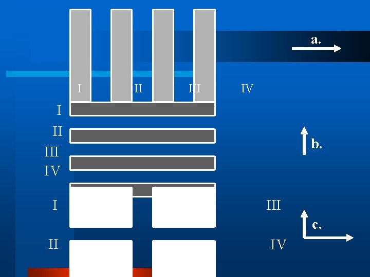
Efficiency of Latin Squares cw RCB Design R(RCB) = [MSr + (t-1)EMS]/(t+1)EMS C(RCB) = [MSc + (t-1)EMS]/(t+1)EMS R(RCB) = 0. 81 : C(RCB) = 3. 66 Latin square in this instance increased precision on 266% over RCB or is less precise if replicates were switched.
a. I II III IV I b. III c. II IV
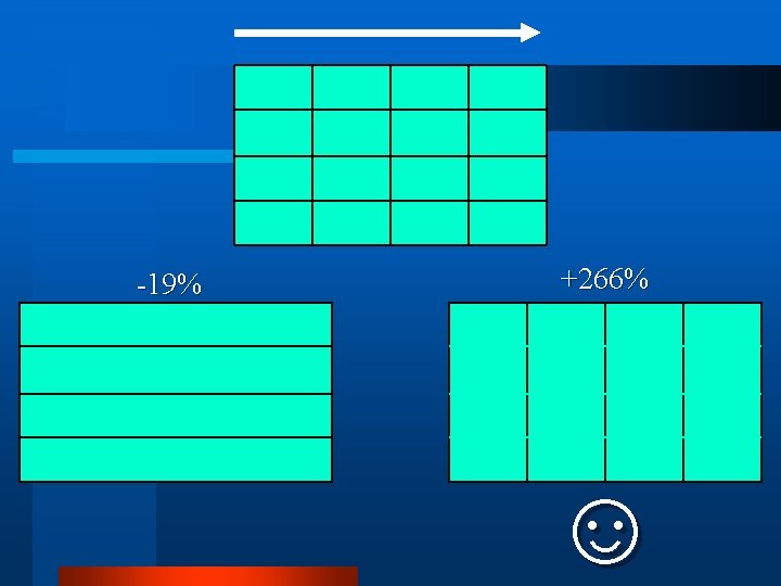
-19% +266% ☺

Analyses of Lattice Squares Yijk = + ri + a bj See Table 5 & 6, Page 105 & 106 + a t k + eijk
Analyses of Lattice Squares v Calculate sub-block totals (b) and replicate totals (R). v Calculate the treatment totals (T) and the grand total (G). v For each treatment, calculate the Bt values which is the sum of all block totals that contain the ith treatment.
Analyses of Lattice Squares v Calculate sub-block totals (b) and replicate totals (R). v Calculate the treatment totals (T) and the grand total (G). v For each treatment, calculate the Bt values which is the sum of all block totals that contain the ith treatment.
Analyses of Lattice Squares v Treatment 5 is in block 2, 5, 10, 15, and 20, so B 5 = 616+639+654+675+827 = 3411. v Note that the sum of the Bt values is G x k, where k is the block size. v For each treatment calculate: W = k. T – (k+1)Bt + G W 5 = 4(816)-(5)(3, 411)+13, 746 = -45
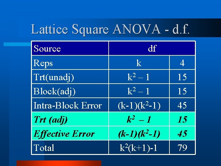
Lattice Square ANOVA - d. f. Source Reps Trt(unadj) Block(adj) Intra-Block Error Trt (adj) Effective Error Total df k k 2 – 1 (k-1)(k 2 -1) k 2(k+1)-1 4 15 15 45 79

Analyses of Lattice Squares v Compute the total correction factor as: CF = (∑xij)2/n CF = G 2/[(k 2)(k+1)] (13, 746)2/(16)(5) 2, 361, 906

Analyses of Lattice Squares v Compute the total SS as: Total SS = xij 2 – CF [1472+1522+…+2252] – 2, 361, 906 = 58, 856

Analyses of Lattice Squares v Compute the replicate block SS as: Replicate SS = R 2/k 2 – CF [25952+27292+…+29252]/16 – 2, 361, 906 = 5, 946
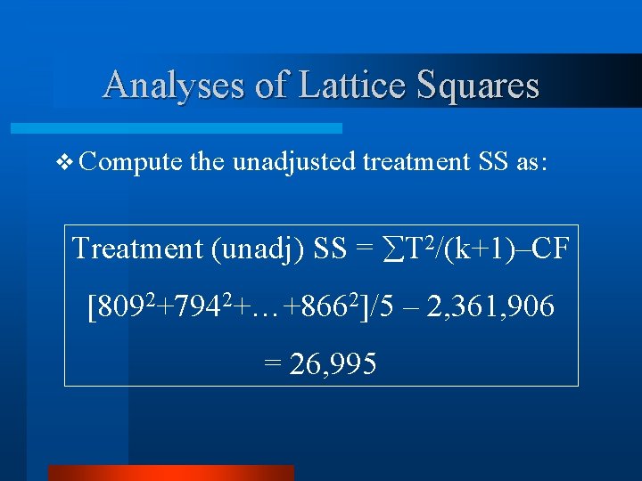
Analyses of Lattice Squares v Compute the unadjusted treatment SS as: Treatment (unadj) SS = T 2/(k+1)–CF [8092+7942+…+8662]/5 – 2, 361, 906 = 26, 995

Analyses of Lattice Squares v Compute the adjusted block SS as: Block (adj) SS = W 2/k 3(k+1) – CF [8092+7942+…+8662]/320 – 2, 361, 906 = 11, 382
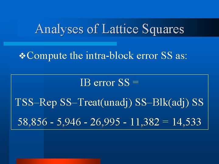
Analyses of Lattice Squares v Compute the intra-block error SS as: IB error SS = TSS–Rep SS–Treat(unadj) SS–Blk(adj) SS 58, 856 - 5, 946 - 26, 995 - 11, 382 = 14, 533

Lattice Square ANOVA v Calculate and IBE. Mean Squares for block(adj) Source Reps T(unadj) Blk(adj) Intra block error df 4 15 15 45 SS 5, 946 26, 995 11, 382 14, 533 MS 1, 486 1, 800 759 323
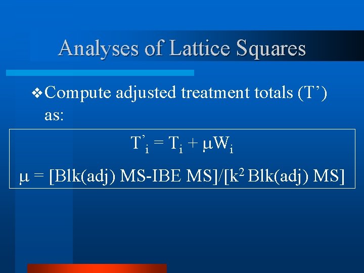
Analyses of Lattice Squares v Compute adjusted treatment totals (T’) as: T’i = Ti + Wi = [Blk(adj) MS-IBE MS]/[k 2 Blk(adj) MS]
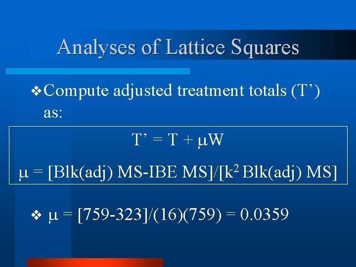
Analyses of Lattice Squares v Compute adjusted treatment totals (T’) as: T’ = T + W = [Blk(adj) MS-IBE MS]/[k 2 Blk(adj) MS] v = [759 -323]/(16)(759) = 0. 0359
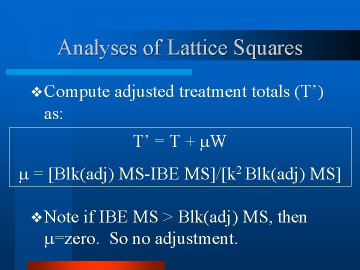
Analyses of Lattice Squares v Compute adjusted treatment totals (T’) as: T’ = T + W = [Blk(adj) MS-IBE MS]/[k 2 Blk(adj) MS] v Note if IBE MS > Blk(adj) MS, then =zero. So no adjustment.
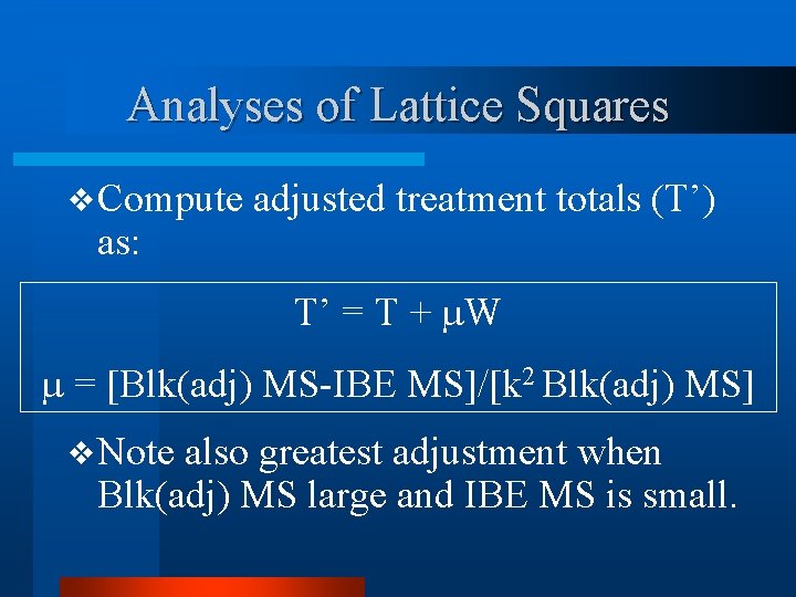
Analyses of Lattice Squares v Compute as: adjusted treatment totals (T’) T’ = T + W = [Blk(adj) MS-IBE MS]/[k 2 Blk(adj) MS] v Note also greatest adjustment when Blk(adj) MS large and IBE MS is small.
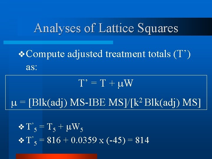
Analyses of Lattice Squares v Compute adjusted treatment totals (T’) as: T’ = T + W = [Blk(adj) MS-IBE MS]/[k 2 Blk(adj) MS] = T 5 + W 5 v T’ 5 = 816 + 0. 0359 x (-45) = 814 v T ’ 5
![Analyses of Lattice Squares v Compute adjusted treatment means (M’) as: M’ = T’/[k+1] Analyses of Lattice Squares v Compute adjusted treatment means (M’) as: M’ = T’/[k+1]](http://slidetodoc.com/presentation_image_h2/3ec68cfa5208881f20fdb70624c8c654/image-43.jpg)
Analyses of Lattice Squares v Compute adjusted treatment means (M’) as: M’ = T’/[k+1]
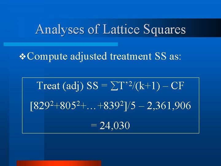
Analyses of Lattice Squares v Compute adjusted treatment SS as: Treat (adj) SS = T’ 2/(k+1) – CF [8292+8052+…+8392]/5 – 2, 361, 906 = 24, 030
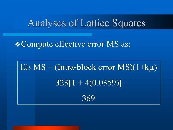
Analyses of Lattice Squares v Compute effective error MS as: EE MS = (Intra-block error MS)(1+k ) 323[1 + 4(0. 0359)] 369
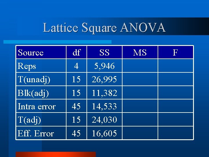
Lattice Square ANOVA Source Reps T(unadj) Blk(adj) Intra error T(adj) Eff. Error df 4 15 15 45 SS 5, 946 26, 995 11, 382 14, 533 24, 030 16, 605 MS F
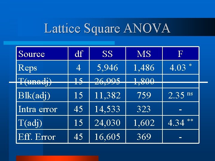
Lattice Square ANOVA Source Reps T(unadj) Blk(adj) Intra error T(adj) Eff. Error df 4 15 15 45 SS 5, 946 26, 995 11, 382 14, 533 24, 030 16, 605 MS 1, 486 1, 800 759 323 1, 602 369 F 4. 03 * 2. 35 ns 4. 34 ** -
![Efficiency of Lattice Design 100 x [Blk(adj)SS+Intra error SS]/k(k 2 -1)EMS 100 [11, 382 Efficiency of Lattice Design 100 x [Blk(adj)SS+Intra error SS]/k(k 2 -1)EMS 100 [11, 382](http://slidetodoc.com/presentation_image_h2/3ec68cfa5208881f20fdb70624c8c654/image-48.jpg)
Efficiency of Lattice Design 100 x [Blk(adj)SS+Intra error SS]/k(k 2 -1)EMS 100 [11, 382 + 14, 533]/4(16)369 117% I II III IV V V
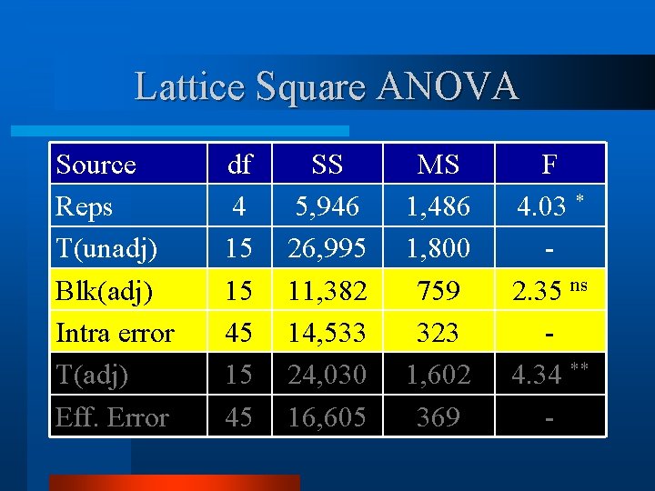
Lattice Square ANOVA Source Reps T(unadj) Blk(adj) Intra error T(adj) Eff. Error df 4 15 15 45 SS 5, 946 26, 995 11, 382 14, 533 24, 030 16, 605 MS 1, 486 1, 800 759 323 1, 602 369 F 4. 03 * 2. 35 ns 4. 34 ** -

RCB ANOVA Source Reps T(unadj) Error df 4 15 60 SS 5, 946 26, 995 25, 915 MS 1, 486 1, 800 432 F 3. 44 * 4. 25 ** -
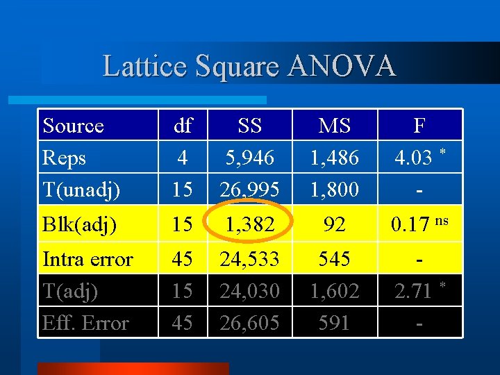
Lattice Square ANOVA Source Reps T(unadj) df 4 15 SS 5, 946 26, 995 MS 1, 486 1, 800 F 4. 03 * - Blk(adj) 15 1, 382 92 0. 17 ns Intra error T(adj) Eff. Error 45 15 45 24, 533 24, 030 26, 605 545 1, 602 591 2. 71 * -
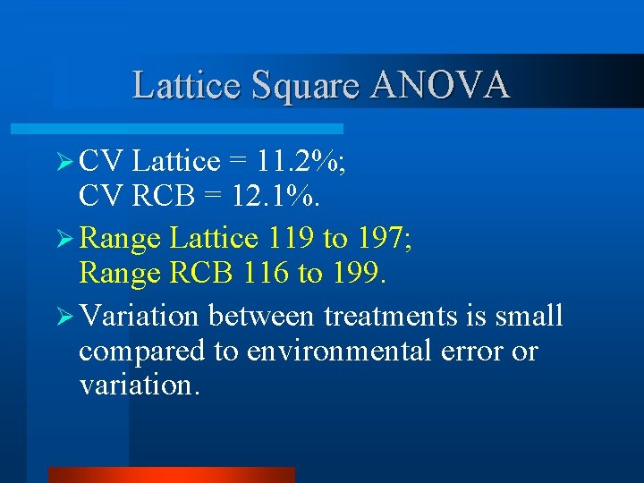
Lattice Square ANOVA Ø CV Lattice = 11. 2%; CV RCB = 12. 1%. Ø Range Lattice 119 to 197; Range RCB 116 to 199. Ø Variation between treatments is small compared to environmental error or variation.
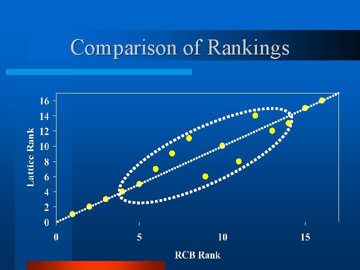
Comparison of Rankings

ANOVA of Factorial Designs
- Slides: 54