An Update on the Stony Brook University Ensemble

An Update on the Stony Brook University Ensemble Forecast System Brian A. Colle, Matthew Jones, Yanluan Lin, and Joseph B. Olson Institute for Terrestrial and Planetary Sciences Stony Brook University / SUNY Jefferey S. Tongue NOAA/NWS Upton, NY

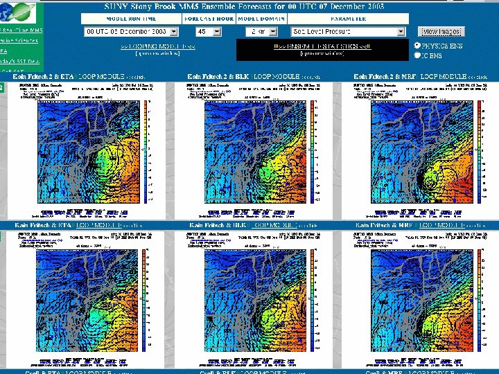
SUNY-SB Realtime MM 5 Domains

Stony Brook Real-time 6 -member 12 km. WRF System ensemble NCEP grids (Eta, GFS, NCEP breds) MM 5 V 3. 6 32 -level, Grell CP (36/12 km), Simple ice, MRF PBL) Web page 60 -h Deterministic Runs (00/12 Z) 48 -h 18 -member MM 5 Ensemble Stony Brook Applications Collaborative Applications MM 5 Verification Wavewatch III Ocean Model (storm surge) Energy Load Forecasts NWS AWIPS NWS-NERFC hydro model BNL- NYC Observatory Computers: 4 -processor Compaq ES 40, 2 -processor DS 20, 10 -node dual Athlon, 15 -node dual Xeon)

Ensemble Objectives Explore the benefits and weakenesses of running a multi-physics and initial condition ensemble over the Northeast at moderately high resolution (12 -km grid spacing). l l Learn how to use ensemble data in operations. Determine how the various physical parameterizations in the ensemble perform during the warm and cool seasons. l
 PHYSICS ENSEMBLE MATRIX")
18 -Member MM 5 Ensemble (00 UTC cycle, 36/12 km domains) PHYSICS ENSEMBLE MATRIX INITIAL CONDITION ENSEMBLE MATRIX (each uses Grell-MRF physical combination)
 Ensemble Mean In a good ensemble, “truth” looks like")
ENSEMBLE BASIC CONCEPTS 1. ) Ensemble Mean In a good ensemble, “truth” looks like a member of the ensemble. Over many simulation periods, the ensemble mean outperforms individual ensemble members in terms of mean-square error (Leith 1974). True solution Mean solution Member trajectories
 Probabilistic forecasts If an ensemble forecast system properly captures the")
BASIC CONCEPTS 2. ) Probabilistic forecasts If an ensemble forecast system properly captures the uncertainty, the ensemble solution will identify the possible weather outcomes, including those with low probability of occurrence, reducing the “element of surprise” (Brooks and Doswell 1993). Mean solution True solution Member trajectories
 Predict forecast skill (reliability) Ensemble spread should be related to")
BASIC CONCEPTS 3. ) Predict forecast skill (reliability) Ensemble spread should be related to ensemble-mean skill. That is, high (low) spread events correspond to low (high) forecast skill (Houtekamer 1993). High skill And confidence Low spread Low skill High spread

Model Surface Temperature Errors Winter Summer Errors in excess of 1. 5ºC dominate portions of the model domain Eta MM 5 ● Model errors have a seasonal dependence ● Temperature error reverses sign at the coast. ● Errors are averages forecast hours 12 -48. Solid contours are positive biases, dashed contours are negative biases. Contour intervals of 0. 5 ºC.
 during the cool season TEMP SLP MRF fix")
48 -h mean errors (at 44004) during the cool season TEMP SLP MRF fix and TOGA COARE FLUX
 1200 UTC 12/6 radar 1200 UTC")
5 -6 December 2003 Nor-easter (the first test) 1200 UTC 12/6 radar 1200 UTC 12/6 surface
 Eta (24 -48 h pcp) GFS")
Operational Model Failure (Hour 48, valid 12/06/12 Z) Eta (24 -48 h pcp) GFS (24 -48 h pcp) MM 5 (45 -48 h pcp) MM 5 (new MRF) 24 12 3 mm mm
 GFS (12")
OBS (12 Z 27 Jan 04 – 12 Z 28 Jan 04) GFS (12 -36 h pcp) mm Eta (12 -36 h pcp) MM 5 Prob cat: 1> 0. 01… 4 =12 -25 mm Darker shading = more confidence in category
 Eta (12")
OBS (12 Z 17 Sep 04 – 12 Z 18 Sep 04) Eta (12 -36 h pcp) Operational model qpf 9/18 case GFS (12 -36 h pcp) mm MM 5 Prob cat: 6=53 -126 mm, 7 > 126

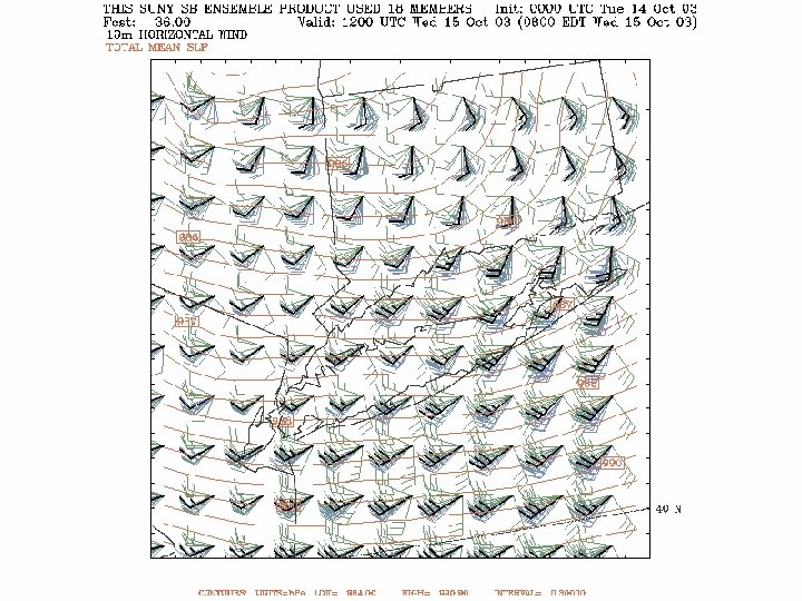
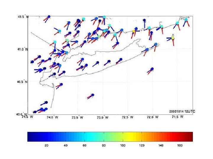
1200 UTC 15 October 2003

Real-time Verification

18 -member MM 5 ensemble MOS using: 6 -hourly data Hourly data Surface temperature ●Suface relative humidity ●Sea-level pressure ●Surface wind speed ●Surface wind direction ●Precipitation ● Climatic data ● cosine(day of year) LW out ●SW out ●LW down ●SW down ●PBL height ●LH flux ●SH flux ● 500 mb geopotential height ●Moisture (upper/mid/low levels) ● 850 mb temperature ● Equations are created for each forecast hour (1 -48), for each variable, for each ensemble member, and for each spatial point of interest. Two month training period (June-July 2003).

Aug-Sept 2003 Temp MAEs Islip, NY Aug-Sept 2003 WSP MAEs 44008 Black: raw model output control member °C m/s Dashed: 6 variable mos; blue: control member MOS, green: mean MOS Solid: 18 variable mos; blue: control member MOS, Dashed: 6 variable mos; Solid: 18 variable mos; blue: control member MOS green: mean MOS forecast hour
 Model in real-time since")
Real-time WRF Modeling Running the Weather and Research Forecast (WRF) Model in real-time since summer 2004 at 36 - and 12 -km grid spacing. l Using Mass coordinate with 32 vertical levels. Control run uses Kain-Fritsch, simple ice (3 -class) micro, Dudhia radiation, and YSU PBL. l Objectives: Compare WRF with MM 5 and Eta at moderate resolution and evaluate WRF for different mesoscale weather. l A 6 member WRF ensemble has been developed by varying some ICs (Eta vs GFS), CPs (K-F vs Grell) and PBLs (YSU vs Eta). The GFS-WRF (YSU-KF) will be run at 4 -km with no Conv Param. and compared with the 5 -km WRF CONUS using Eta for ICs for the NCEP/FSL winter experiment. l

MM 5 vs WRF: 2100 UTC 23 July 2004 12 -km MM 5 18 -21 Z precip 12 -km WRF 18 -21 Z precip Both runs used Grell, MRF PBL, and simple ice
 WRF (Grell and YSU PBL)")
0000 UTC 20 October 2004 (12 -km hour 48) WRF (Grell and YSU PBL) WRF (KF and YSU PBL) Spurious bulls-eyes over water
 WRF Grell-YSU (Conv pcp)")
0000 UTC 20 October 2004 (12 -km, hours 45 -48) WRF Grell-YSU (Conv pcp) WRF Grell (explicit pcp)

Summary and Future Work An ensemble MM 5 forecast system has been developed. For the evening forecast cycle, 18 separate forecasts are generated using different initializations and model physics. See http: //fractus. msrc. sunysb. edu/mm 5 rte l The 12 -km ensemble is has been expanded to include a 6 -member Weather and Research Forecasting (WRF) model. Will help complement the deterministic NCEP/FSL 5 -km WRF Winter Forecast Experiment over the CONUS. l The ensemble system has proved to be a useful addition to the NCEP model suite. l Future work will explore benefits of ensemble post-processing as well additional ensemble diversification using different initial conditions (MM 5/WRF breds, NOGAPS, and CMC ICs). l
- Slides: 26