An overview of iterative reconstruction applied to PET

An overview of iterative reconstruction applied to PET (and SPECT)? Professor Brian F Hutton Institute of Nuclear Medicine University College London brian. hutton@uclh. nhs. uk m

Outline • Understanding iterative reconstruction (ML-EM + OS-EM) • the flexibility in system modelling • modelling resolution • time-of-flight m

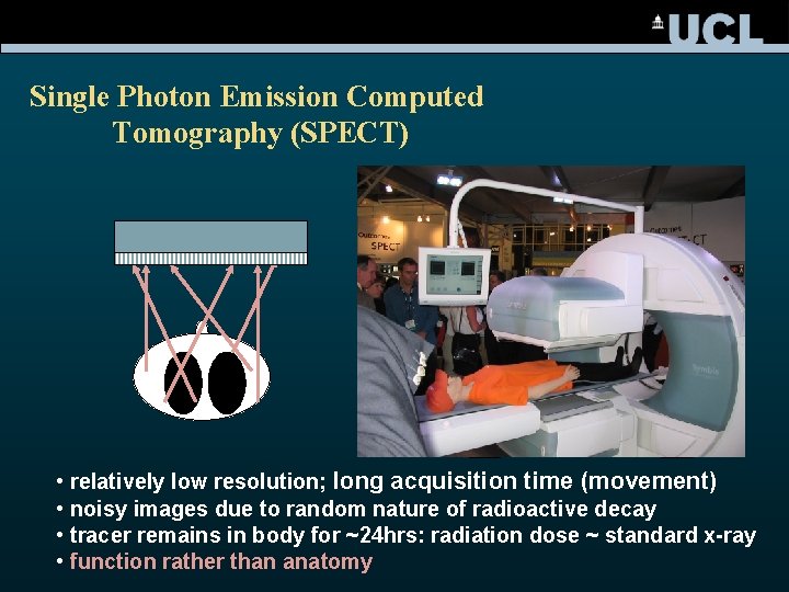
Single Photon Emission Computed Tomography (SPECT) • relatively low resolution; long acquisition time (movement) • noisy images due to random nature of radioactive decay • tracer remains in body for ~24 hrs: radiation dose ~ standard x-ray • function rather than anatomy

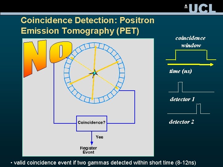
Coincidence Detection: Positron Emission Tomography (PET) coincidence window time (ns) detector 1 detector 2 • valid coincidence event if two gammas detected within short time (8 -12 ns)

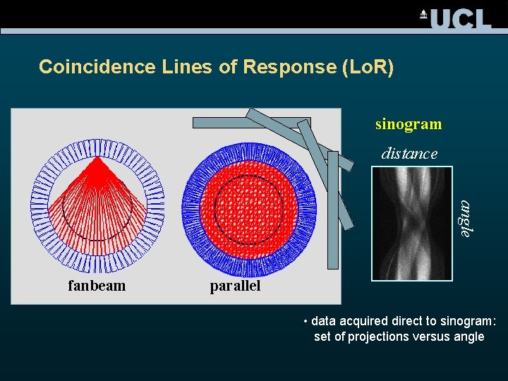
Coincidence Lines of Response (Lo. R) sinogram distance angle fanbeam parallel • data acquired direct to sinogram: set of projections versus angle

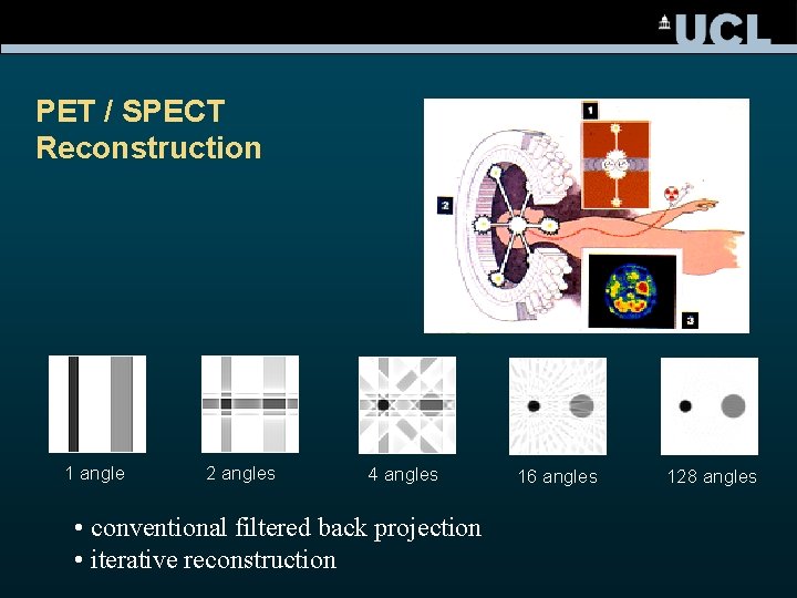
PET / SPECT Reconstruction 1 angle 2 angles 4 angles • conventional filtered back projection • iterative reconstruction 16 angles 128 angles

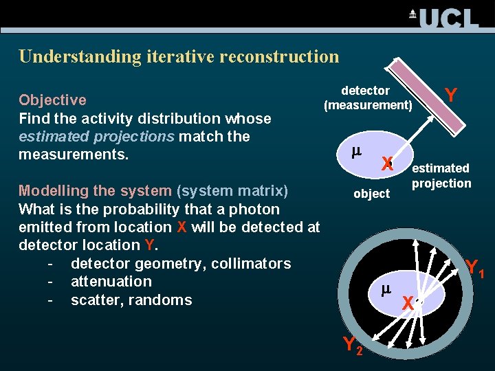
Understanding iterative reconstruction Objective Find the activity distribution whose estimated projections match the measurements. Modelling the system (system matrix) What is the probability that a photon emitted from location X will be detected at detector location Y. - detector geometry, collimators - attenuation - scatter, randoms detector (measurement) m X object m Y 2 Y estimated projection Y 1 X

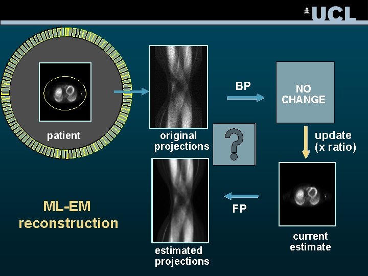
BP patient update (x ratio) original projections ML-EM reconstruction NO original CHANGE estimate FP estimated projections current estimate

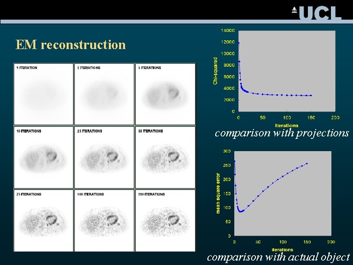
EM reconstruction comparison with projections comparison with actual object

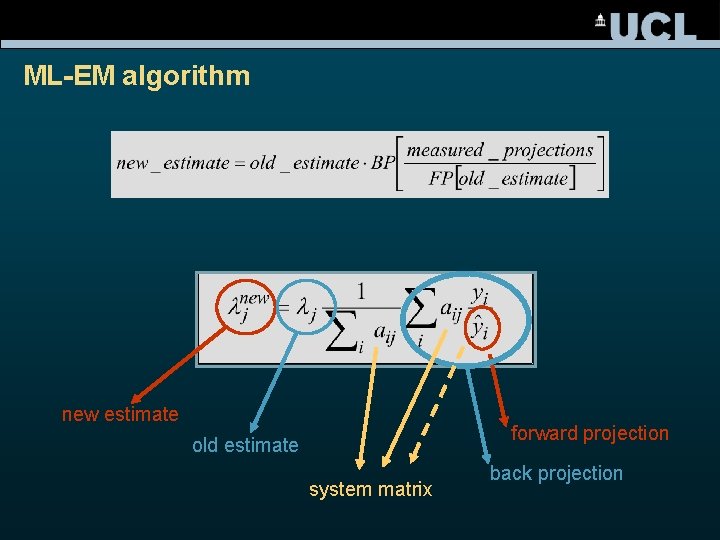
ML-EM algorithm new estimate forward projection old estimate system matrix back projection

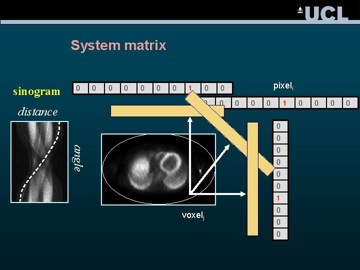
System matrix sinogram 0 distance 0 0 0 1 0 0 pixeli 0 0 0 1 0 0 angle 0 0 1 voxelj 0 0 0 0

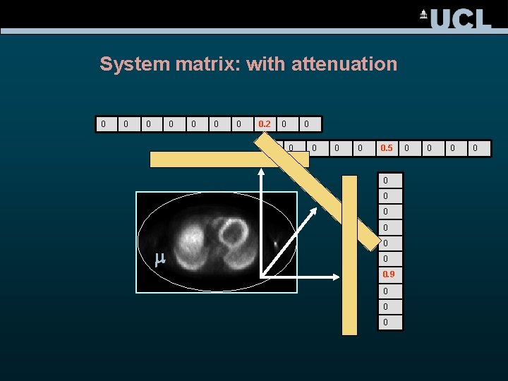
System matrix: with attenuation 0 0 0 0. 2 0 0 0 0. 5 0 0 m 0 0 0. 9 0 0 0 0

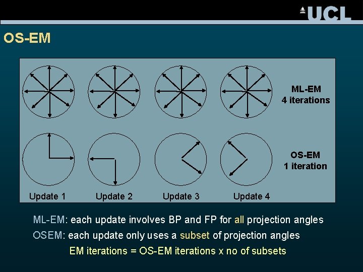
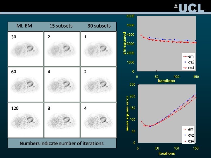
OS-EM ML-EM 4 iterations OS-EM 1 iteration Update 1 Update 2 Update 3 Update 4 ML-EM: each update involves BP and FP for all projection angles OSEM: each update only uses a subset of projection angles EM iterations = OS-EM iterations x no of subsets

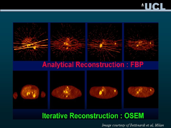
Image courtesy of Bettinardi et al, Milan

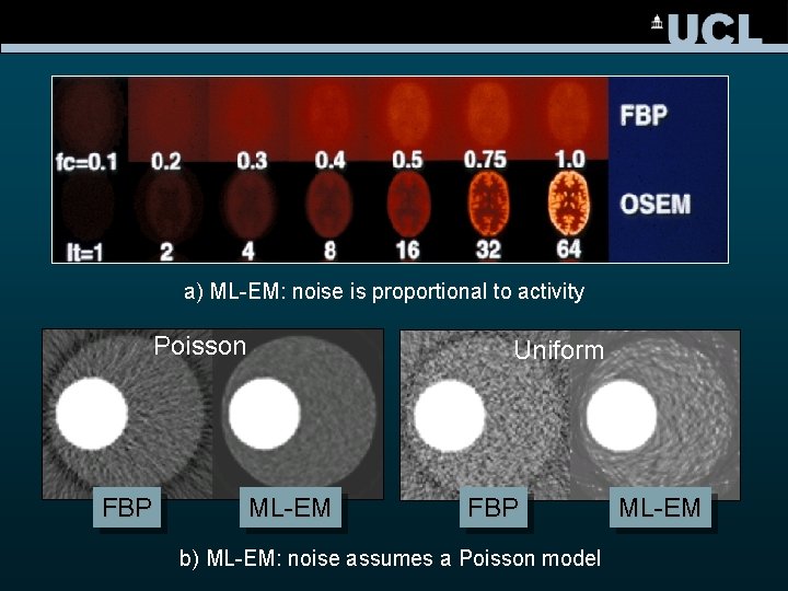
a) ML-EM: noise is proportional to activity Poisson FBP Uniform ML-EM FBP b) ML-EM: noise assumes a Poisson model ML-EM

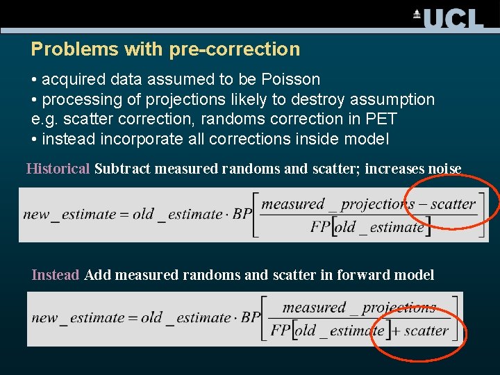
Problems with pre-correction • acquired data assumed to be Poisson • processing of projections likely to destroy assumption e. g. scatter correction, randoms correction in PET • instead incorporate all corrections inside model Historical Subtract measured randoms and scatter; increases noise Instead Add measured randoms and scatter in forward model

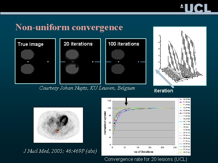
Non-uniform convergence True image 20 iterations 100 iterations Courtesy Johan Nuyts, KU Leuven, Belgium iteration J Nucl Med, 2005; 46: 469 P (abs) Convergence rate for 20 lesions (UCL)

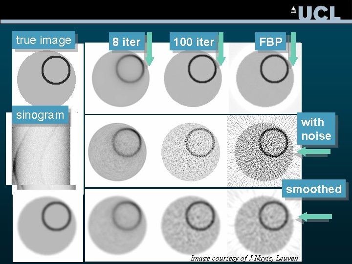
true image 8 iter 100 iter FBP sinogram with noise smoothed Image courtesy of J Nuyts, Leuven

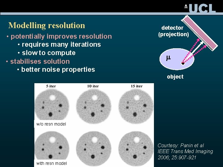
Modelling resolution • potentially improves resolution • requires many iterations • slow to compute • stabilises solution • better noise properties detector (projection) m object w/o resn model Courtesy: Panin et al IEEE Trans Med Imaging 2006; 25: 907 -921 with resn model

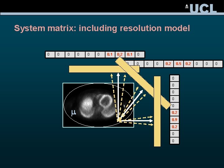
System matrix: including resolution model 0 0 0 0. 1 0. 2 0. 1 0 0 0. 2 0. 5 0 0 m 0 0. 2 0. 9 0. 2 0 0 0

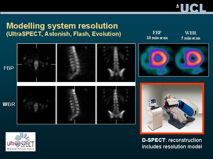
Modelling system resolution (Ultra. SPECT, Astonish, Flash, Evolution) FBP WBR 10 min scan 5 min scan FBP WBR D-SPECT: reconstruction includes resolution model

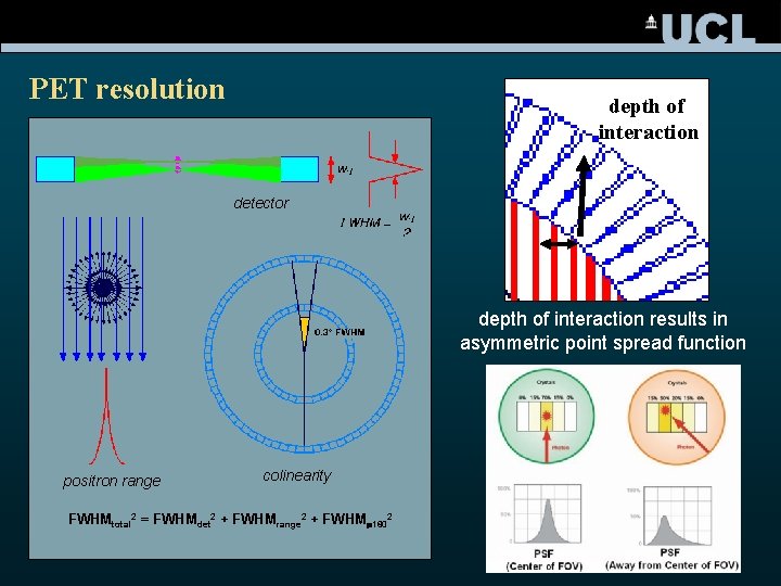
PET resolution depth of interaction detector fan depth of interaction results in asymmetric point spread function positron range colinearity FWHMtotal 2 = FWHMdet 2 + FWHMrange 2 + FWHM 1802

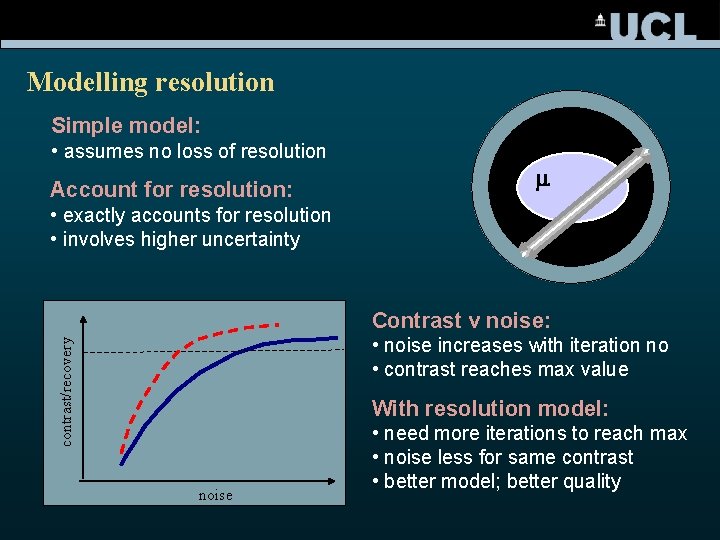
Modelling resolution Simple model: • assumes no loss of resolution Account for resolution: m • exactly accounts for resolution • involves higher uncertainty Contrast v noise: contrast/recovery • noise increases with iteration no • contrast reaches max value With resolution model: noise • need more iterations to reach max • noise less for same contrast • better model; better quality

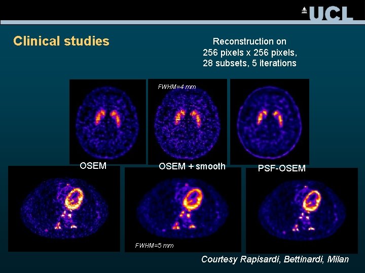
Clinical studies Reconstruction on 256 pixels x 256 pixels, 28 subsets, 5 iterations FWHM=4 mm OSEM + smooth PSF-OSEM FWHM=5 mm Courtesy Rapisardi, Bettinardi, Milan

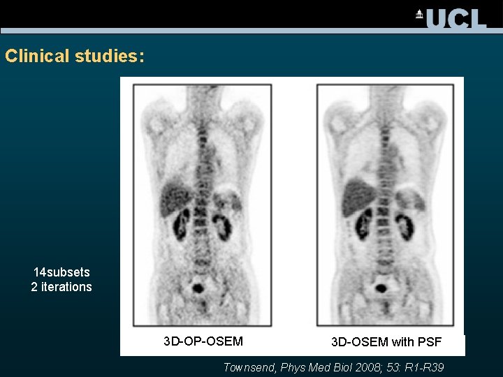
Clinical studies: 14 subsets 2 iterations 3 D-OP-OSEM 3 D-OSEM with PSF Townsend, Phys Med Biol 2008; 53: R 1 -R 39

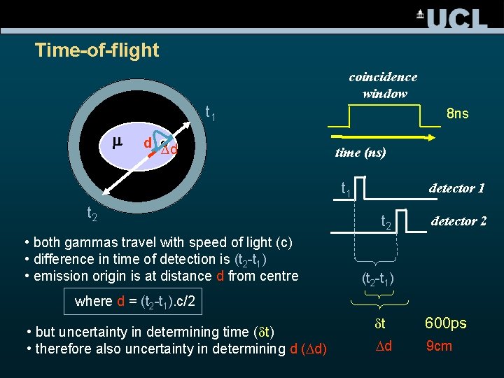
Time-of-flight coincidence window t 1 m d Dd 8 ns time (ns) t 1 t 2 • both gammas travel with speed of light (c) • difference in time of detection is (t 2 -t 1) • emission origin is at distance d from centre detector 1 t 2 detector 2 (t 2 -t 1) where d = (t 2 -t 1). c/2 • but uncertainty in determining time (dt) • therefore also uncertainty in determining d (Dd) dt 600 ps Dd 9 cm

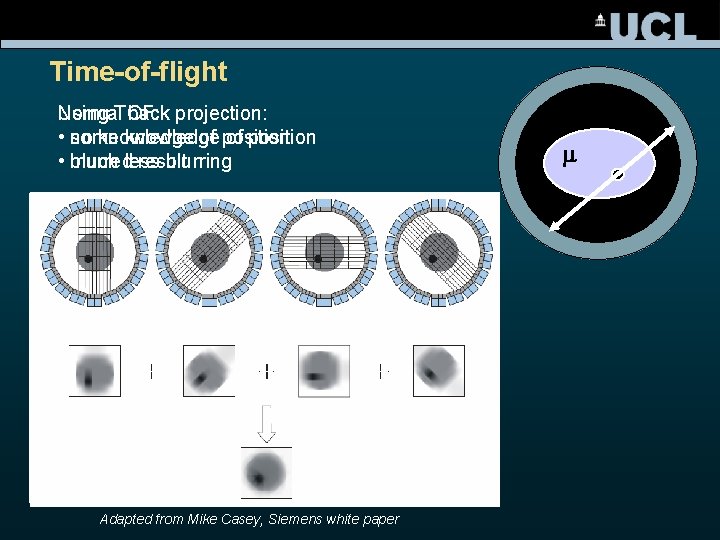
Time-of-flight Normal back projection: Using TOF: • no knowledge of position some knowledge of position • blurred result much less blurring Adapted from Mike Casey, Siemens white paper m

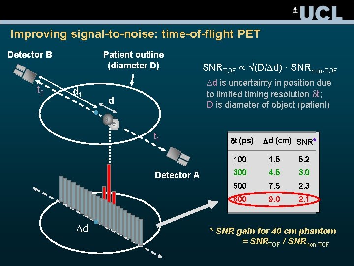
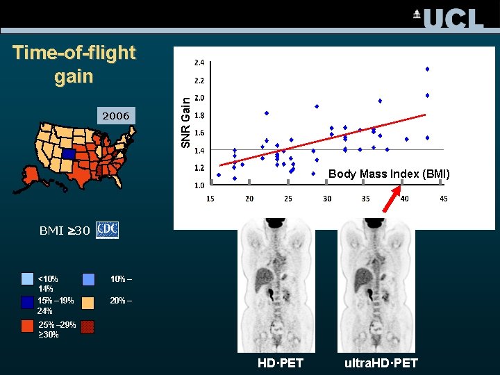
Improving signal-to-noise: time-of-flight PET Detector B t 2 Patient outline (diameter D) d 1 SNRTOF √(D/Dd) · SNRnon-TOF Dd is uncertainty in position due to limited timing resolution dt; D is diameter of object (patient) d e+ e t 1 Detector A Dd dt (ps) Dd (cm) SNR* 100 1. 5 5. 2 300 4. 5 3. 0 500 7. 5 2. 3 600 9. 0 2. 1 * SNR gain for 40 cm phantom = SNRTOF / SNRnon-TOF

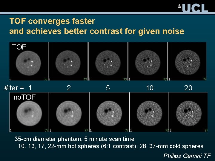
TOF converges faster and achieves better contrast for given noise TOF #iter = 1 no. TOF 2 5 10 20 35 -cm diameter phantom; 5 minute scan time 10, 13, 17, 22 -mm hot spheres (6: 1 contrast); 28, 37 -mm cold spheres Philips Gemini TF

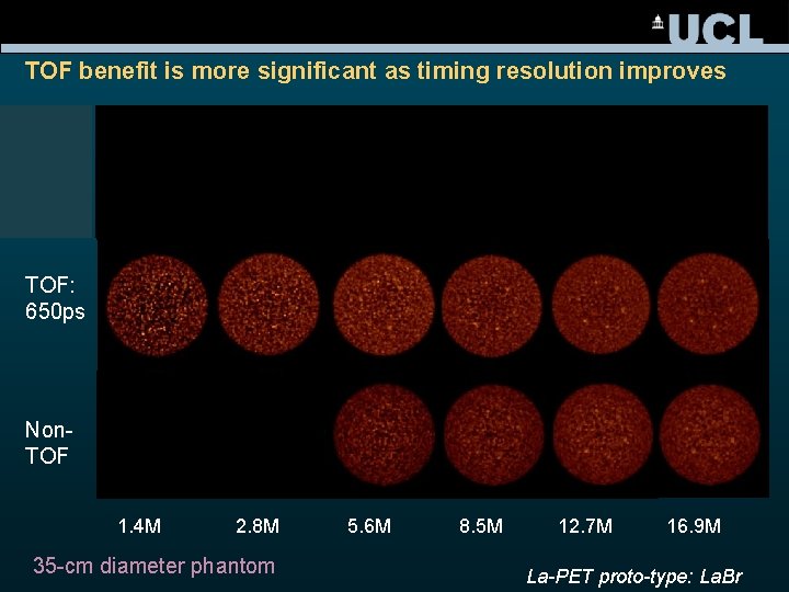
TOF benefit is more significant as timing resolution improves TOF: 400 ps TOF: 650 ps Non. TOF 1. 4 M 2. 8 M 35 -cm diameter phantom 5. 6 M 8. 5 M 12. 7 M 16. 9 M La-PET proto-type: La. Br

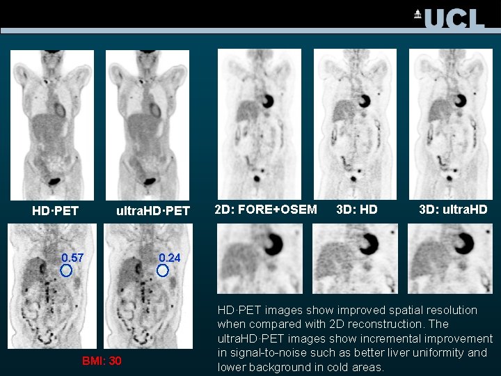
HD·PET ultra. HD·PET 0. 57 BMI: 30 2 D: FORE+OSEM 3 D: HD 3 D: ultra. HD 0. 24 HD·PET images show improved spatial resolution when compared with 2 D reconstruction. The ultra. HD·PET images show incremental improvement in signal-to-noise such as better liver uniformity and lower background in cold areas.

2006 1990 SNR Gain Time-of-flight gain Body Mass Index (BMI) BMI 30 <10% 14% 15%– 19% 24% 10%– 25%– 29% ≥ 30% HD·PET ultra. HD·PET

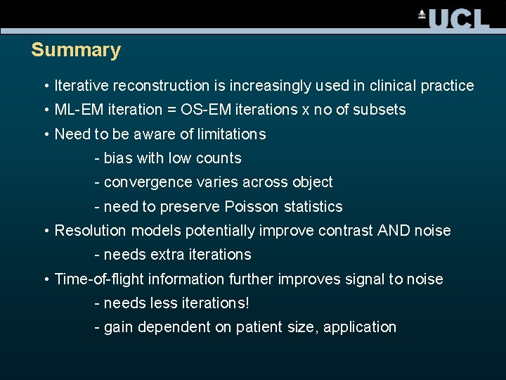
Summary • Iterative reconstruction is increasingly used in clinical practice • ML-EM iteration = OS-EM iterations x no of subsets • Need to be aware of limitations - bias with low counts - convergence varies across object - need to preserve Poisson statistics • Resolution models potentially improve contrast AND noise - needs extra iterations • Time-of-flight information further improves signal to noise - needs less iterations! - gain dependent on patient size, application

Acknowledgements Thanks to Joel Karp, Dave Townsend, Johan Nuyts for use of material for slides.

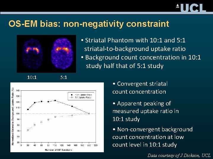
OS-EM bias: non-negativity constraint • Striatal Phantom with 10: 1 and 5: 1 striatal-to-background uptake ratio • Background count concentration in 10: 1 study half that of 5: 1 study 10: 1 5: 1 • Convergent striatal count concentration • Apparent peaking of measured uptake ratio in 10: 1 study • Non-convergent background count concentration at low count level in 10: 1 study Data courtesy of J Dickson, UCL

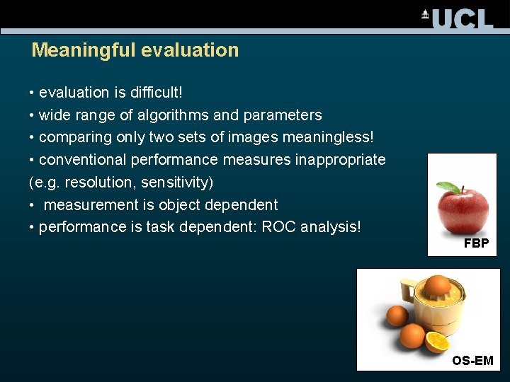
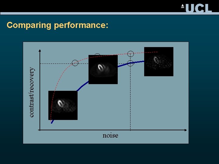
Meaningful evaluation • evaluation is difficult! • wide range of algorithms and parameters • comparing only two sets of images meaningless! • conventional performance measures inappropriate (e. g. resolution, sensitivity) • measurement is object dependent • performance is task dependent: ROC analysis! FBP OS-EM

contrast/recovery Comparing performance: noise

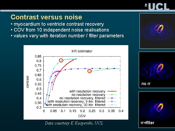
Contrast versus noise • myocardium to ventricle contrast recovery • COV from 10 independent noise realisations • values vary with iteration number / filter parameters no rr Data courtesy K Kacperski, UCL rr+filter