An Introduction to the Expectation Maximization EM Algorithm

An Introduction to the Expectation. Maximization (EM) Algorithm CSE 802, Spring 2006 Department of Computer Science and Engineering Michigan State University 1

Overview • The problem of missing data • A mixture of Gaussian • The EM Algorithm – The Q-function, the E-step and the M-step • Some examples • Summary 2

Missing Data • Data collection and feature generation are not perfect. Objects in a pattern recognition application may have missing features – In the classification problem of sea bass versus salmon, the lightness feature can still be estimated if part of the fish is occluded. This is not so for the width feature – Features are extracted by multiple sensors. One or multiple sensors may be malfunctioning when the object is presented – A respondent fails to answer all the questions in a questionnaire – Some participants quit during the middle of a study, where measurements are taken at different time points • An example of missing data: “dermatology” from UCI Missing values 3

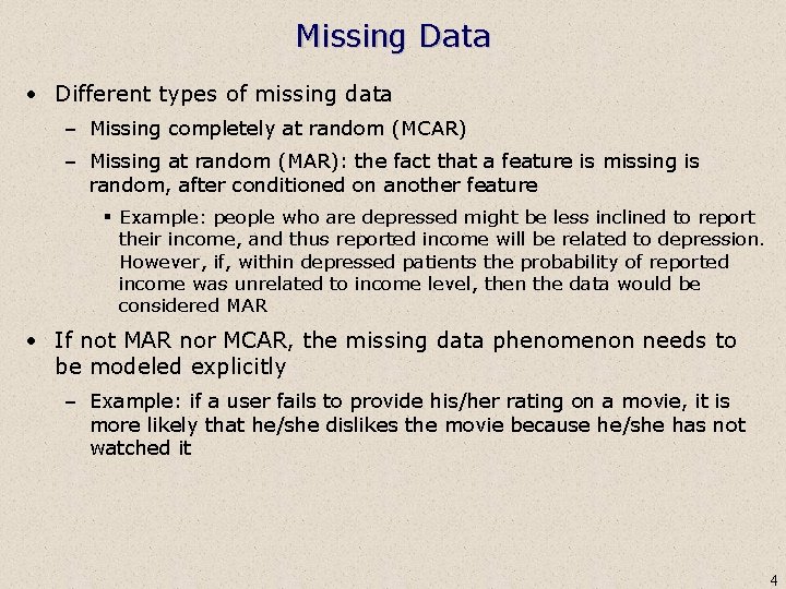
Missing Data • Different types of missing data – Missing completely at random (MCAR) – Missing at random (MAR): the fact that a feature is missing is random, after conditioned on another feature § Example: people who are depressed might be less inclined to report their income, and thus reported income will be related to depression. However, if, within depressed patients the probability of reported income was unrelated to income level, then the data would be considered MAR • If not MAR nor MCAR, the missing data phenomenon needs to be modeled explicitly – Example: if a user fails to provide his/her rating on a movie, it is more likely that he/she dislikes the movie because he/she has not watched it 4

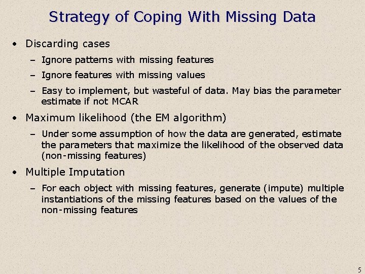
Strategy of Coping With Missing Data • Discarding cases – Ignore patterns with missing features – Ignore features with missing values – Easy to implement, but wasteful of data. May bias the parameter estimate if not MCAR • Maximum likelihood (the EM algorithm) – Under some assumption of how the data are generated, estimate the parameters that maximize the likelihood of the observed data (non-missing features) • Multiple Imputation – For each object with missing features, generate (impute) multiple instantiations of the missing features based on the values of the non-missing features 5

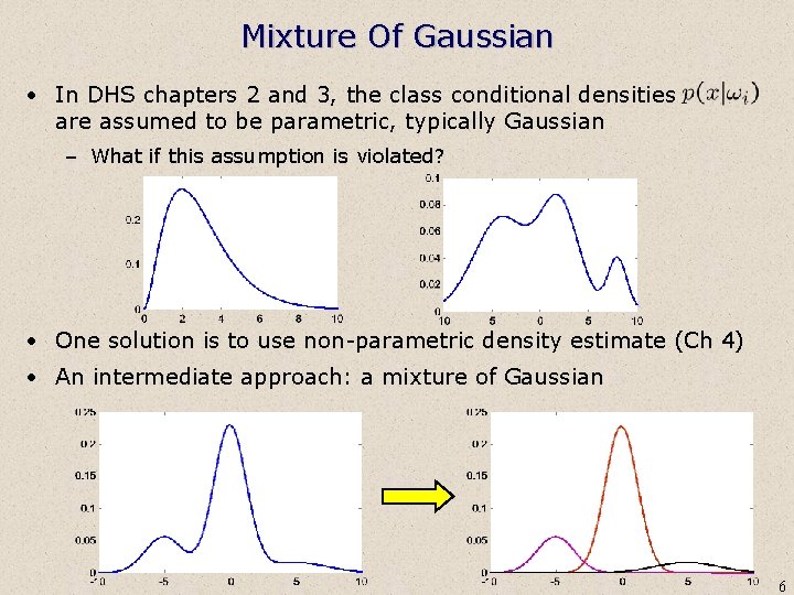
Mixture Of Gaussian • In DHS chapters 2 and 3, the class conditional densities are assumed to be parametric, typically Gaussian – What if this assumption is violated? • One solution is to use non-parametric density estimate (Ch 4) • An intermediate approach: a mixture of Gaussian 6

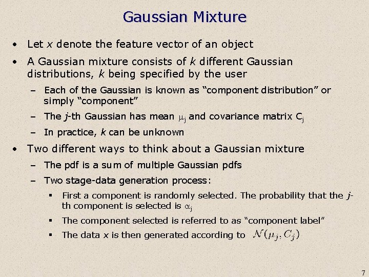
Gaussian Mixture • Let x denote the feature vector of an object • A Gaussian mixture consists of k different Gaussian distributions, k being specified by the user – Each of the Gaussian is known as “component distribution” or simply “component” – The j-th Gaussian has mean mj and covariance matrix Cj – In practice, k can be unknown • Two different ways to think about a Gaussian mixture – The pdf is a sum of multiple Gaussian pdfs – Two stage-data generation process: § First a component is randomly selected. The probability that the jth component is selected is aj § The component selected is referred to as “component label” § The data x is then generated according to 7

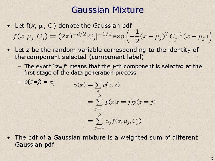
Gaussian Mixture • Let f(x, mj, Cj) denote the Gaussian pdf • Let z be the random variable corresponding to the identity of the component selected (component label) – The event “z=j” means that the j-th component is selected at the first stage of the data generation process – p(z=j) = aj • The pdf of a Gaussian mixture is a weighted sum of different Gaussian pdf 8

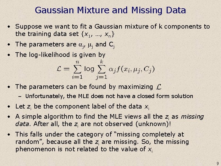
Gaussian Mixture and Missing Data • Suppose we want to fit a Gaussian mixture of k components to the training data set {x 1, …, xn} • The parameters are aj, mj and Cj • The log-likelihood is given by • The parameters can be found by maximizing – Unfortunately, the MLE does not have a closed form solution • Let zi be the component label of the data xi • A simple algorithm to find the MLE views all the zi as missing data. After all, the zi are not observed (unknown)! • This falls under the category of “missing completely at random”, because all the zi are missing. So, the missing phenomenon is not related to the value of xi 9

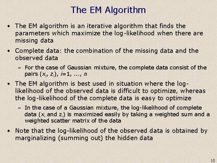
The EM Algorithm • The EM algorithm is an iterative algorithm that finds the parameters which maximize the log-likelihood when there are missing data • Complete data: the combination of the missing data and the observed data – For the case of Gaussian mixture, the complete data consist of the pairs (xi, zi), i=1, . . . , n • The EM algorithm is best used in situation where the loglikelihood of the observed data is difficult to optimize, whereas the log-likelihood of the complete data is easy to optimize – In the case of a Gaussian mixture, the log-likelihood of complete data (xi and zi) is maximized easily by taking a weighted sum and a weighted scatter matrix of the data • Note that the log-likelihood of the observed data is obtained by marginalizing (summing out) the hidden data 10

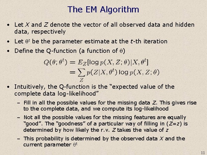
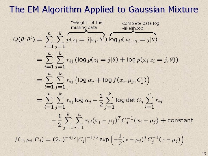
The EM Algorithm • Let X and Z denote the vector of all observed data and hidden data, respectively • Let qt be the parameter estimate at the t-th iteration • Define the Q-function (a function of q) • Intuitively, the Q-function is the “expected value of the complete data log-likelihood” – Fill in all the possible values for the missing data Z. This gives rise to the complete data, and we compute its log-likelihood – Not all the possible values for the missing features are equally “good”. The “goodness” of a particular way of filling in (Z=z) is determined by how likely the r. v. Z takes the value of z – This probability is determined by the observed data X and the current parameter qt 11

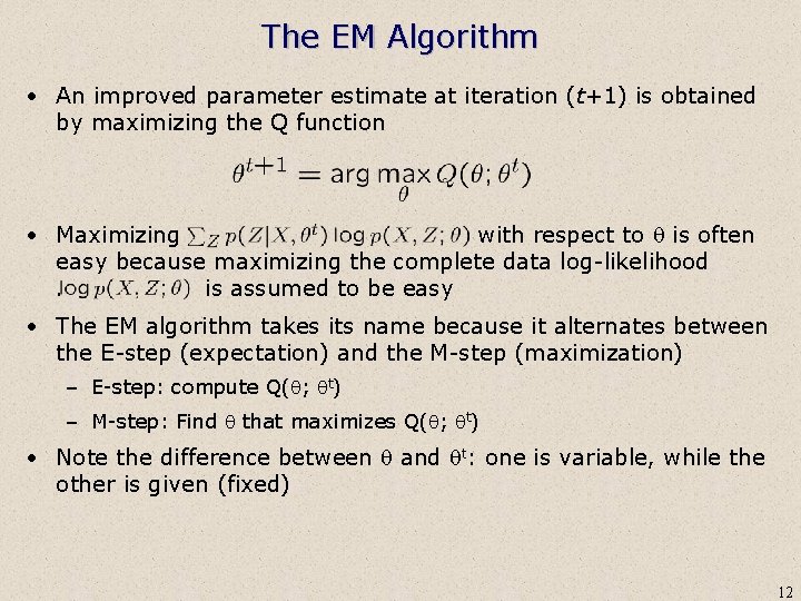
The EM Algorithm • An improved parameter estimate at iteration (t+1) is obtained by maximizing the Q function • Maximizing with respect to q is often easy because maximizing the complete data log-likelihood . is assumed to be easy • The EM algorithm takes its name because it alternates between the E-step (expectation) and the M-step (maximization) – E-step: compute Q(q; qt) – M-step: Find q that maximizes Q(q; qt) • Note the difference between q and qt: one is variable, while the other is given (fixed) 12

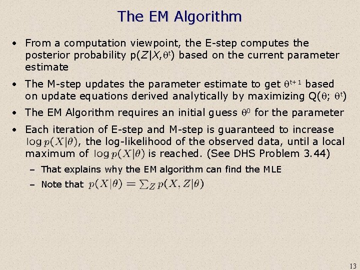
The EM Algorithm • From a computation viewpoint, the E-step computes the posterior probability p(Z|X, qt) based on the current parameter estimate • The M-step updates the parameter estimate to get qt+1 based on update equations derived analytically by maximizing Q(q; qt) • The EM Algorithm requires an initial guess q 0 for the parameter • Each iteration of E-step and M-step is guaranteed to increase , the log-likelihood of the observed data, until a local maximum of is reached. (See DHS Problem 3. 44). – That explains why the EM algorithm can find the MLE – Note that 13

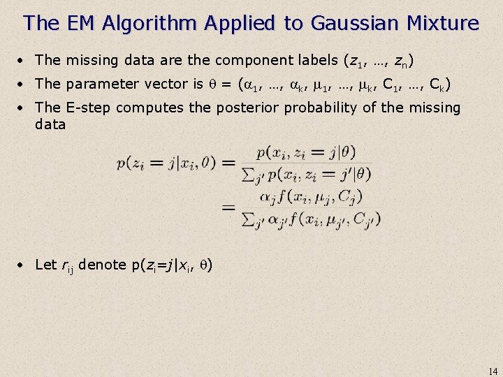
The EM Algorithm Applied to Gaussian Mixture • The missing data are the component labels (z 1, …, zn) • The parameter vector is q = (a 1, …, ak, m 1, …, mk, C 1, …, Ck) • The E-step computes the posterior probability of the missing data • Let rij denote p(zi=j|xi, q) 14

The EM Algorithm Applied to Gaussian Mixture “Weight” of the missing data Complete data log -likelihood 15

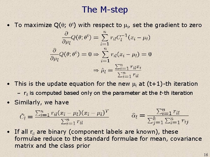
The M-step • To maximize Q(q; qt) with respect to ml, set the gradient to zero • This is the update equation for the new ml at (t+1)-th iteration – ril is computed based only on the parameter at the t-th iteration • Similarly, we have • If all ril are binary (component labels are known), these formulae reduce to the standard formulae for mean, covariance matrix and the class prior 16

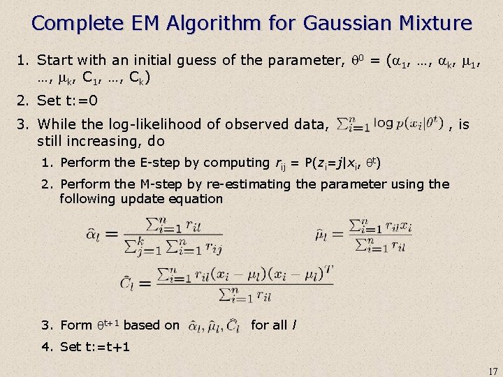
Complete EM Algorithm for Gaussian Mixture 1. Start with an initial guess of the parameter, q 0 = (a 1, …, ak, m 1, …, mk, C 1, …, Ck) 2. Set t: =0 3. While the log-likelihood of observed data, , is still increasing, do 1. Perform the E-step by computing rij = P(zi=j|xi, qt) 2. Perform the M-step by re-estimating the parameter using the following update equation 3. Form qt+1 based on for all l 4. Set t: =t+1 17

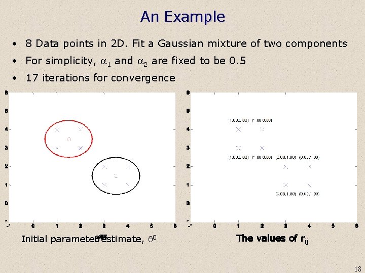
An Example • 8 Data points in 2 D. Fit a Gaussian mixture of two components • For simplicity, a 1 and a 2 are fixed to be 0. 5 • 17 iterations for convergence 10 15 3 11 16 6 5 2 1 8 4 17 14 13 9 7 0 q 12 Initial parameter estimate, q The values of rij 18

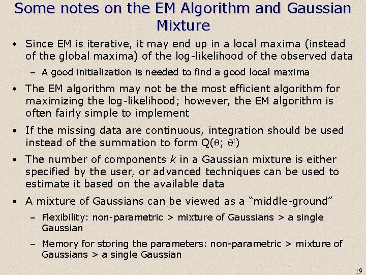
Some notes on the EM Algorithm and Gaussian Mixture • Since EM is iterative, it may end up in a local maxima (instead of the global maxima) of the log-likelihood of the observed data – A good initialization is needed to find a good local maxima • The EM algorithm may not be the most efficient algorithm for maximizing the log-likelihood; however, the EM algorithm is often fairly simple to implement • If the missing data are continuous, integration should be used instead of the summation to form Q(q; qt) • The number of components k in a Gaussian mixture is either specified by the user, or advanced techniques can be used to estimate it based on the available data • A mixture of Gaussians can be viewed as a “middle-ground” – Flexibility: non-parametric > mixture of Gaussians > a single Gaussian – Memory for storing the parameters: non-parametric > mixture of Gaussians > a single Gaussian 19

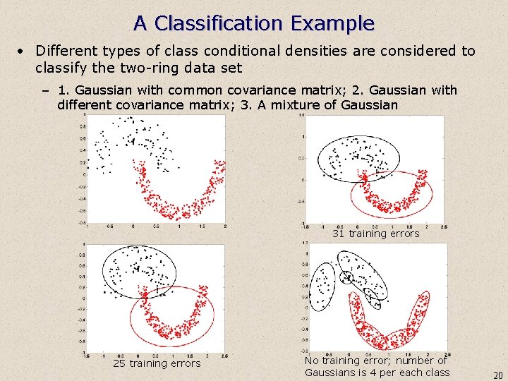
A Classification Example • Different types of class conditional densities are considered to classify the two-ring data set – 1. Gaussian with common covariance matrix; 2. Gaussian with different covariance matrix; 3. A mixture of Gaussian 31 training errors 25 training errors No training error; number of Gaussians is 4 per each class 20

Summary • The problem of missing data is regularly encountered in realworld applications • Instead of discarding the cases with missing data, the EM algorithm can be used to maximize the marginalized loglikelihood (the log-likelihood of data observed) • A mixture of Gaussians provides more flexibility than a single Gaussian for density estimation • By regarding the component labels as missing data, the EM algorithm can be used for parameter estimation in a mixture of Gaussians • The EM algorithm is an iterative algorithm that consists of the E -step (computation of the Q function) and the M-step (maximization of the Q function) 21

References • http: //www. uvm. edu/~dhowell/Stat. Pages/More_Stuff/Missing_ Data/Missing. html • An EM implementation in Matlab: http: //www. cse. msu. edu/~lawhiu/software/em. m • http: //www. lshtm. ac. uk/msu/missingdata/index. html • DHS chapter 3. 9 • Some recent derivations of the EM algorithm in new scenarios • M. Figueiredo, "Bayesian image segmentation using wavelet-based priors", IEEE Computer Society Conference on Computer Vision and Pattern Recognition - CVPR'2005. • B. Krishnapuram, A. Hartemink, L. Carin, and M. Figueiredo, "A Bayesian approach to joint feature selection and classifier design", TPAMI, vol. 26, no. 9, pp. 1105 -1111, 2004. • M. Figueiredo and A. K. Jain, "Unsupervised learning of finite mixture models", TPAMI, vol. 24, no. 3, pp. 381 -396, March 2002. http: //www. lx. it. pt/~mtf/mixturecode. zip for the software 22