An Introduction to Stata for Survey Data Analysis

An Introduction to Stata for Survey Data Analysis Olivier Dupriez, World Bank 2018

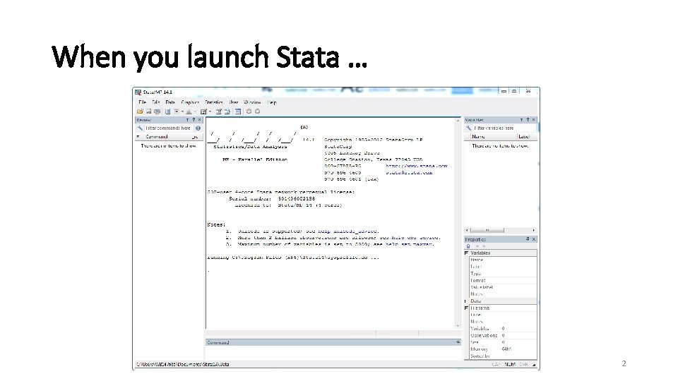
When you launch Stata … 2

Three ways of executing Stata commands • Menus and dialogs (the Graphical User Interface) • The command line • Writing programs (do files) 3

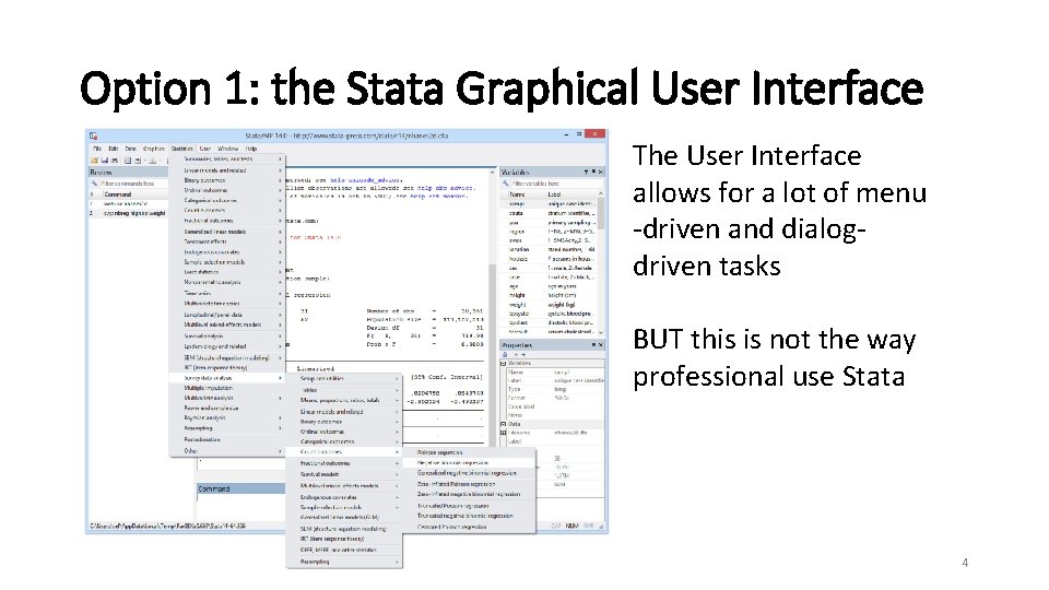
Option 1: the Stata Graphical User Interface The User Interface allows for a lot of menu -driven and dialogdriven tasks BUT this is not the way professional use Stata 4

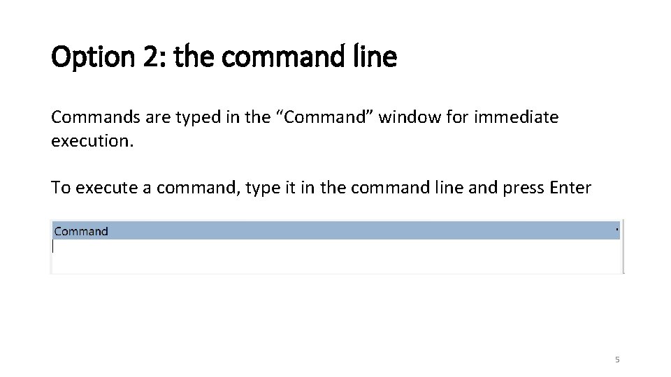
Option 2: the command line Commands are typed in the “Command” window for immediate execution. To execute a command, type it in the command line and press Enter 5

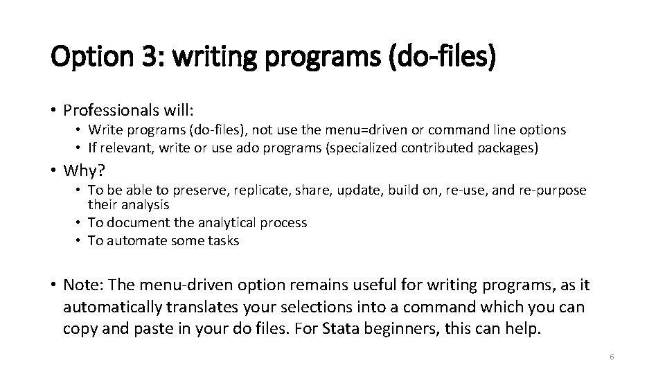
Option 3: writing programs (do files) • Professionals will: • Write programs (do-files), not use the menu=driven or command line options • If relevant, write or use ado programs (specialized contributed packages) • Why? • To be able to preserve, replicate, share, update, build on, re-use, and re-purpose their analysis • To document the analytical process • To automate some tasks • Note: The menu-driven option remains useful for writing programs, as it automatically translates your selections into a command which you can copy and paste in your do files. For Stata beginners, this can help. 6

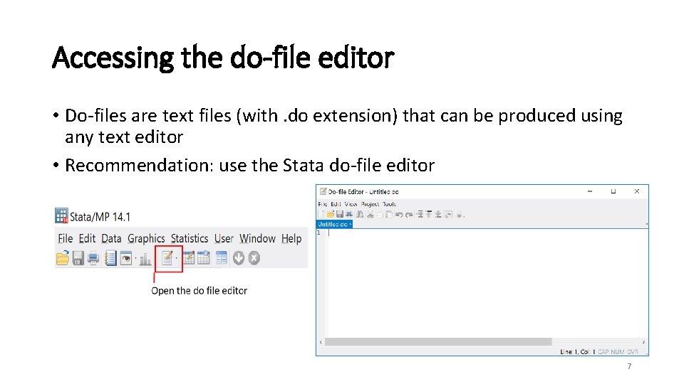
Accessing the do file editor • Do-files are text files (with. do extension) that can be produced using any text editor • Recommendation: use the Stata do-file editor 7

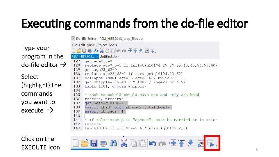
Executing commands from the do file editor Type your program in the do-file editor Select (highlight) the commands you want to execute Click on the EXECUTE icon 8

Ado files (contributed packages) 9

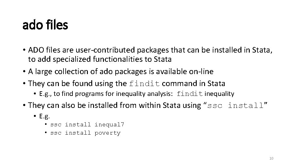
ado files • ADO files are user-contributed packages that can be installed in Stata, to add specialized functionalities to Stata • A large collection of ado packages is available on-line • They can be found using the findit command in Stata • E. g. , to find programs for inequality analysis: findit inequality • They can also be installed from within Stata using “ssc install” • E. g. • ssc install inequal 7 • ssc install poverty 10

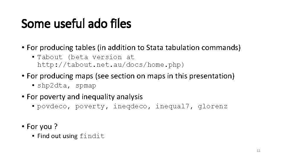
Some useful ado files • For producing tables (in addition to Stata tabulation commands) • Tabout (beta version at http: //tabout. net. au/docs/home. php) • For producing maps (see section on maps in this presentation) • shp 2 dta, spmap • For poverty and inequality analysis • povdeco, poverty, ineqdeco, inequal 7, glorenz • For you ? • Find out using findit 11

Before we start… 12

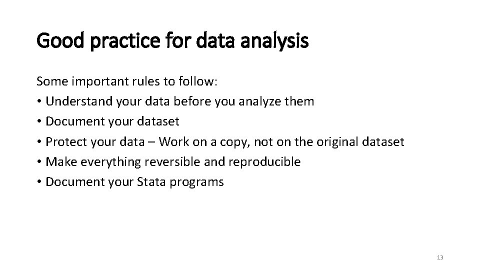
Good practice for data analysis Some important rules to follow: • Understand your data before you analyze them • Document your dataset • Protect your data – Work on a copy, not on the original dataset • Make everything reversible and reproducible • Document your Stata programs 13

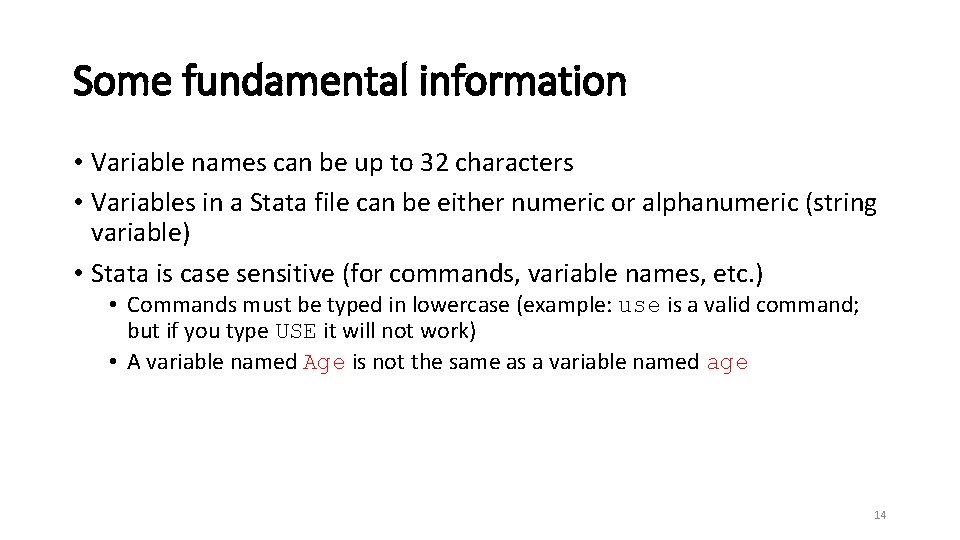
Some fundamental information • Variable names can be up to 32 characters • Variables in a Stata file can be either numeric or alphanumeric (string variable) • Stata is case sensitive (for commands, variable names, etc. ) • Commands must be typed in lowercase (example: use is a valid command; but if you type USE it will not work) • A variable named Age is not the same as a variable named age 14

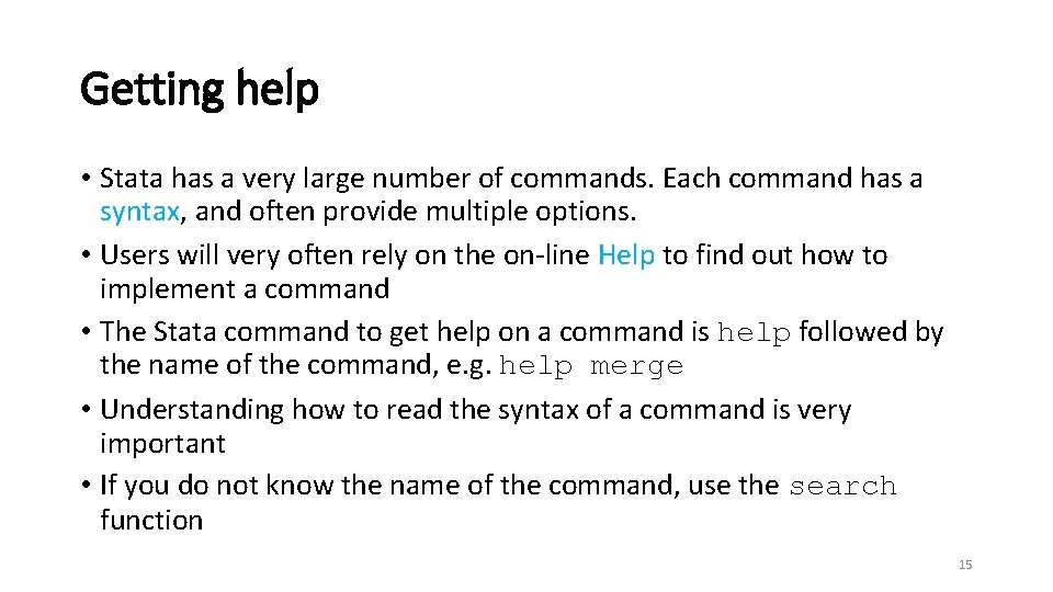
Getting help • Stata has a very large number of commands. Each command has a syntax, and often provide multiple options. • Users will very often rely on the on-line Help to find out how to implement a command • The Stata command to get help on a command is help followed by the name of the command, e. g. help merge • Understanding how to read the syntax of a command is very important • If you do not know the name of the command, use the search function 15

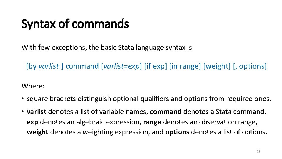
Syntax of commands With few exceptions, the basic Stata language syntax is [by varlist: ] command [varlist=exp] [if exp] [in range] [weight] [, options] Where: • square brackets distinguish optional qualifiers and options from required ones. • varlist denotes a list of variable names, command denotes a Stata command, exp denotes an algebraic expression, range denotes an observation range, weight denotes a weighting expression, and options denotes a list of options. 16

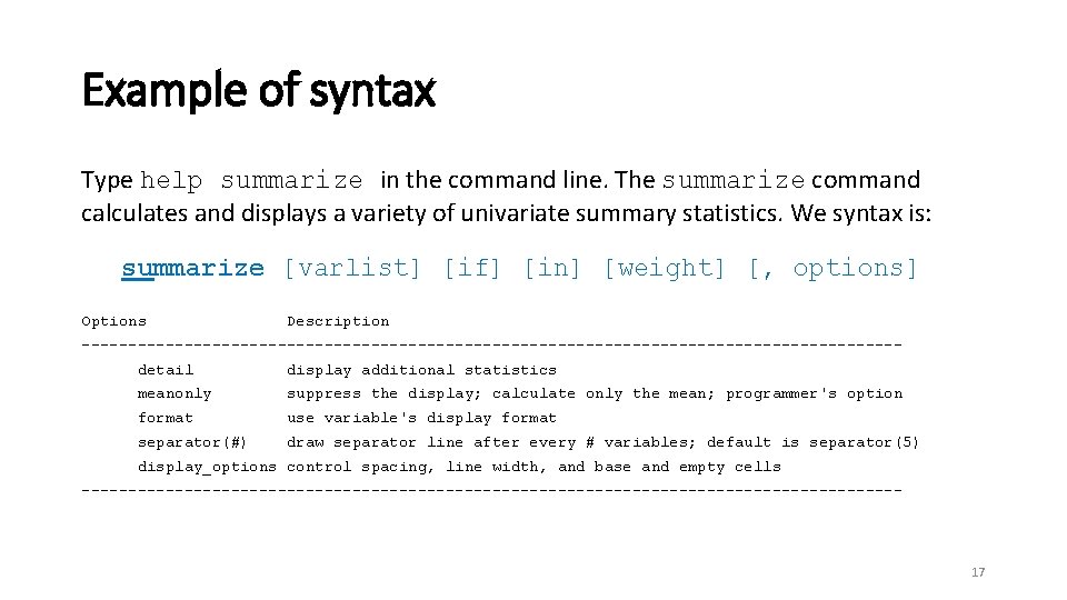
Example of syntax Type help summarize in the command line. The summarize command calculates and displays a variety of univariate summary statistics. We syntax is: summarize [varlist] [if] [in] [weight] [, options] Options Description --------------------------------------------detail display additional statistics meanonly suppress the display; calculate only the mean; programmer's option format use variable's display format separator(#) draw separator line after every # variables; default is separator(5) display_options control spacing, line width, and base and empty cells -------------------------------------------- 17

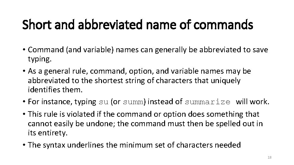
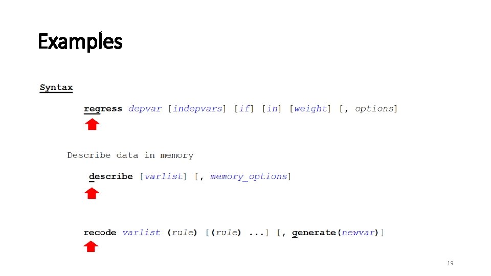
Short and abbreviated name of commands • Command (and variable) names can generally be abbreviated to save typing. • As a general rule, command, option, and variable names may be abbreviated to the shortest string of characters that uniquely identifies them. • For instance, typing su (or summ) instead of summarize will work. • This rule is violated if the command or option does something that cannot easily be undone; the command must then be spelled out in its entirety. • The syntax underlines the minimum set of characters needed 18

Examples 19

Analysis of sample survey data: Survey design, sample weights, and the svy commands 20

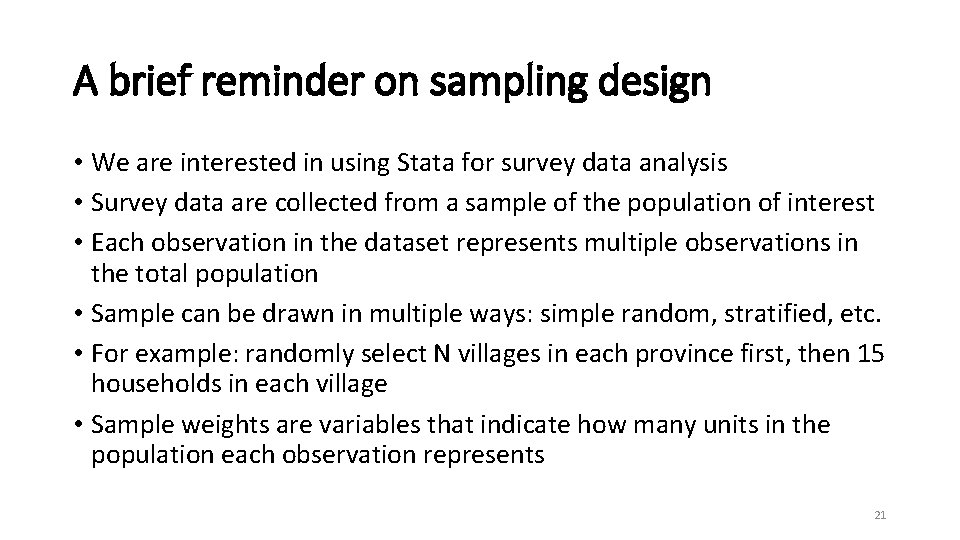
A brief reminder on sampling design • We are interested in using Stata for survey data analysis • Survey data are collected from a sample of the population of interest • Each observation in the dataset represents multiple observations in the total population • Sample can be drawn in multiple ways: simple random, stratified, etc. • For example: randomly select N villages in each province first, then 15 households in each village • Sample weights are variables that indicate how many units in the population each observation represents 21

Sampling weights • Sample weights are typically the inverse of the probability for an observation of being selected • Example: in a simple random selection, if the total population has 1, 000 households and we draw a sample of 5, 000: • The probability of being selected is 5, 000 / 1, 000 = 0. 005 • The sample weight of each household will be 1, 000 / 5, 000 = 200 • In more complex sample designs, the sample weight will be different for each region, or enumeration area, etc. • When we produce estimates (of totals, means, ratios, etc. ) we need to apply these weights to have estimates that represent the population and not the sample (i. e. we need “weighted estimates”) 22

Working on data files 23

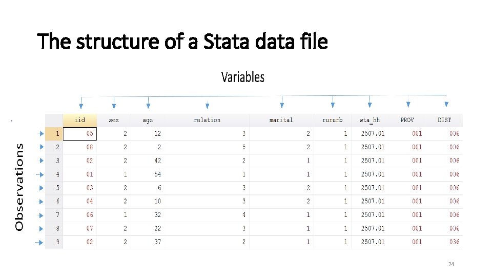
The structure of a Stata data file 24

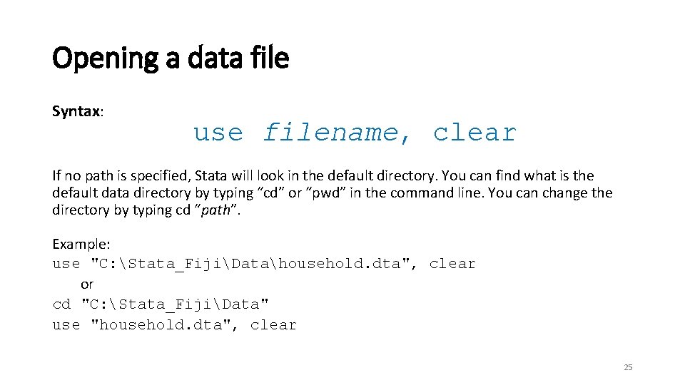
Opening a data file Syntax: use filename, clear If no path is specified, Stata will look in the default directory. You can find what is the default data directory by typing “cd” or “pwd” in the command line. You can change the directory by typing cd “path”. Example: use "C: Stata_FijiDatahousehold. dta", clear or cd "C: Stata_FijiData" use "household. dta", clear 25

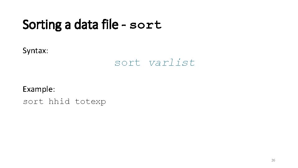
Sorting a data file sort Syntax: sort varlist Example: sort hhid totexp 26

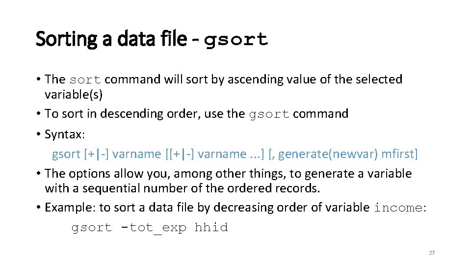
Sorting a data file gsort • The sort command will sort by ascending value of the selected variable(s) • To sort in descending order, use the gsort command • Syntax: gsort [+|-] varname [[+|-] varname. . . ] [, generate(newvar) mfirst] • The options allow you, among other things, to generate a variable with a sequential number of the ordered records. • Example: to sort a data file by decreasing order of variable income: gsort -tot_exp hhid 27

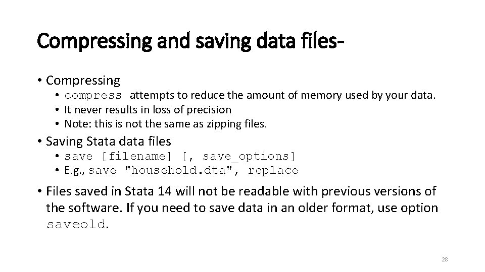
Compressing and saving data files • Compressing • compress attempts to reduce the amount of memory used by your data. • It never results in loss of precision • Note: this is not the same as zipping files. • Saving Stata data files • save [filename] [, save_options] • E. g. , save "household. dta", replace • Files saved in Stata 14 will not be readable with previous versions of the software. If you need to save data in an older format, use option saveold. 28

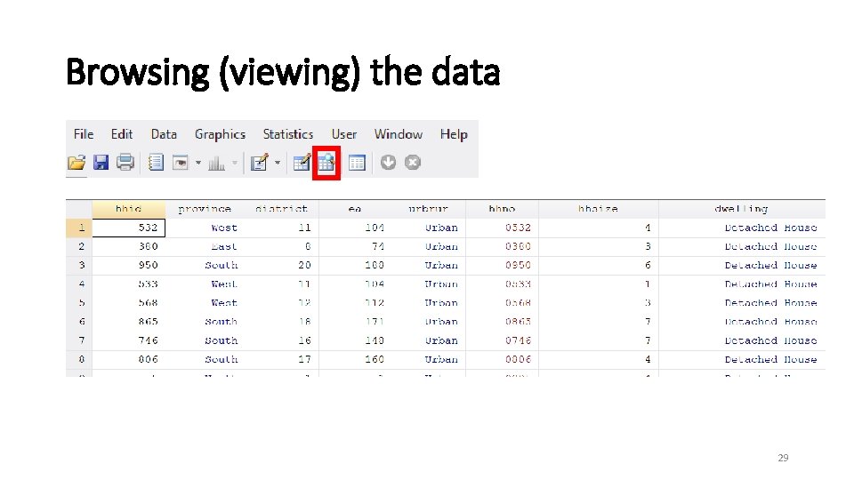
Browsing (viewing) the data 29

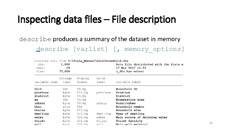
Inspecting data files – File description describe produces a summary of the dataset in memory describe [varlist] [, memory_options] 30

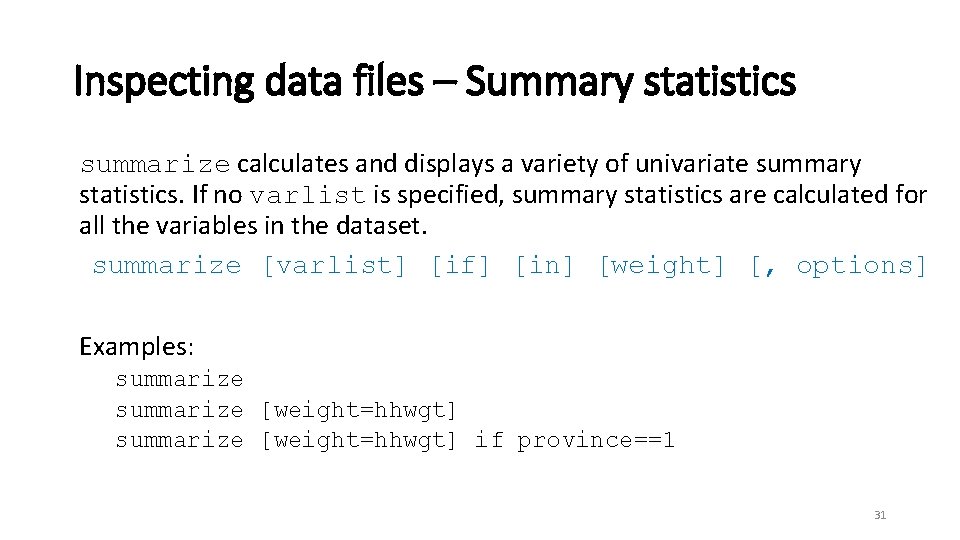
Inspecting data files – Summary statistics summarize calculates and displays a variety of univariate summary statistics. If no varlist is specified, summary statistics are calculated for all the variables in the dataset. summarize [varlist] [if] [in] [weight] [, options] Examples: summarize [weight=hhwgt] if province==1 31

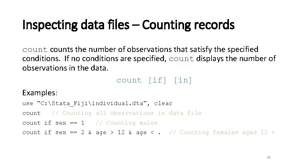
Inspecting data files – Counting records counts the number of observations that satisfy the specified conditions. If no conditions are specified, count displays the number of observations in the data. count [if] [in] Examples: use "C: Stata_Fijiindividual. dta", clear count // Counting all observations in data file count if sex == 1 // Counting males count if sex == 2 & age > 12 & age <. // Counting females aged 12 + 32

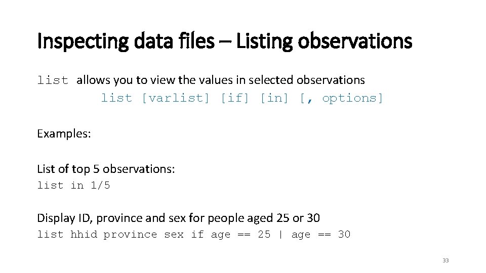
Inspecting data files – Listing observations list allows you to view the values in selected observations list [varlist] [if] [in] [, options] Examples: List of top 5 observations: list in 1/5 Display ID, province and sex for people aged 25 or 30 list hhid province sex if age == 25 | age == 30 33

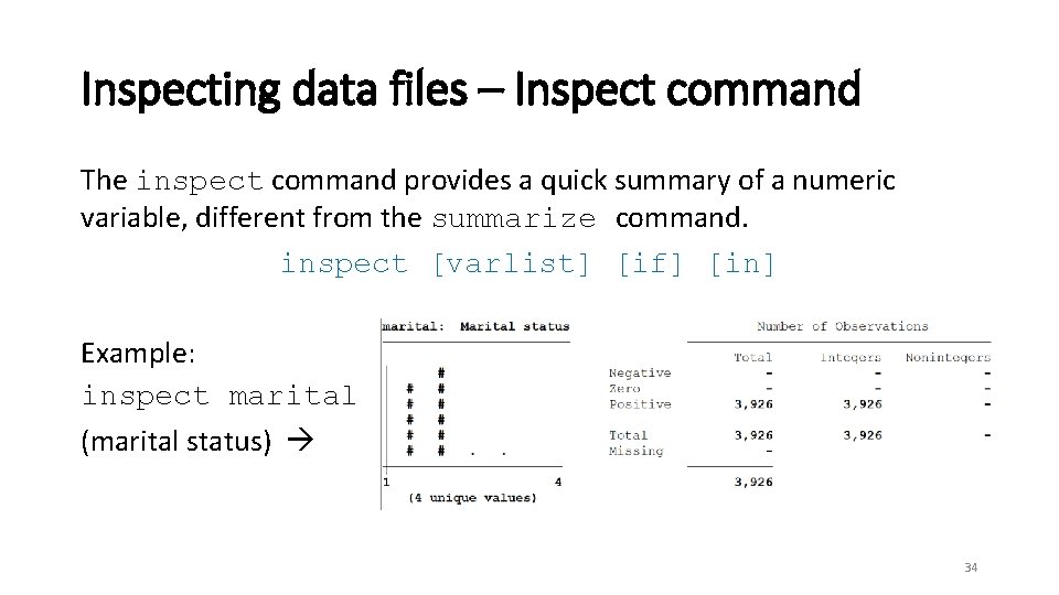
Inspecting data files – Inspect command The inspect command provides a quick summary of a numeric variable, different from the summarize command. inspect [varlist] [if] [in] Example: inspect marital (marital status) 34

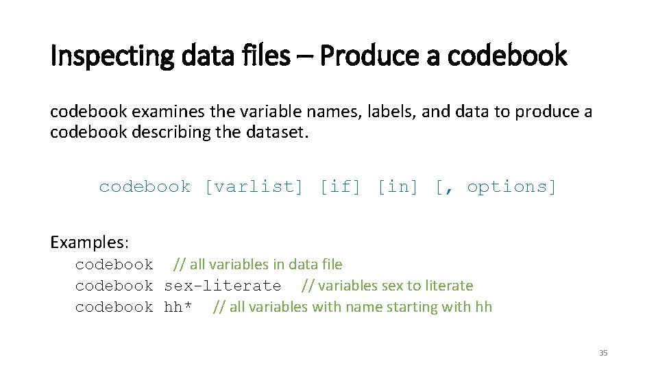
Inspecting data files – Produce a codebook examines the variable names, labels, and data to produce a codebook describing the dataset. codebook [varlist] [if] [in] [, options] Examples: codebook // all variables in data file codebook sex-literate // variables sex to literate codebook hh* // all variables with name starting with hh 35

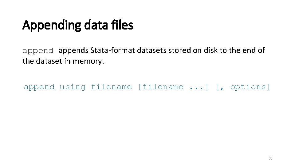
Appending data files appends Stata-format datasets stored on disk to the end of the dataset in memory. append using filename [filename. . . ] [, options] 36

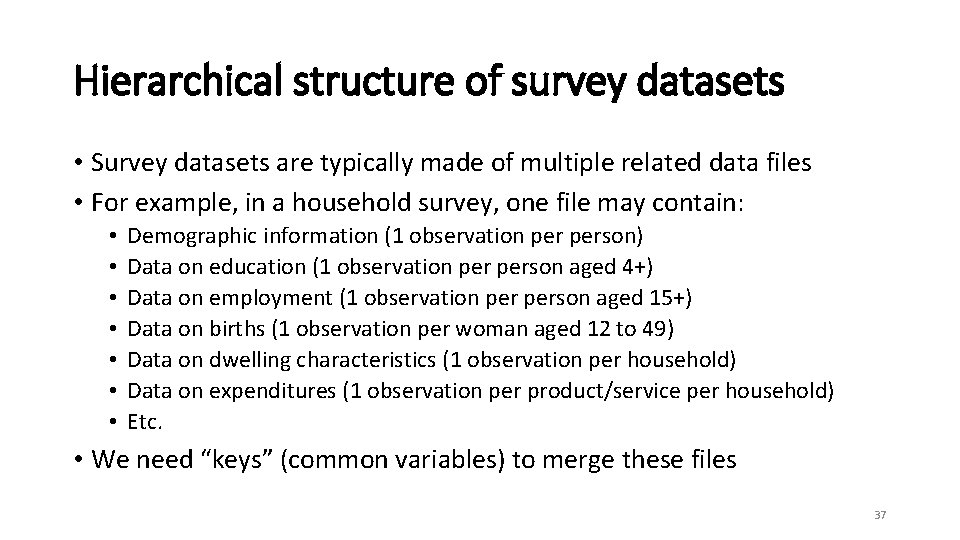
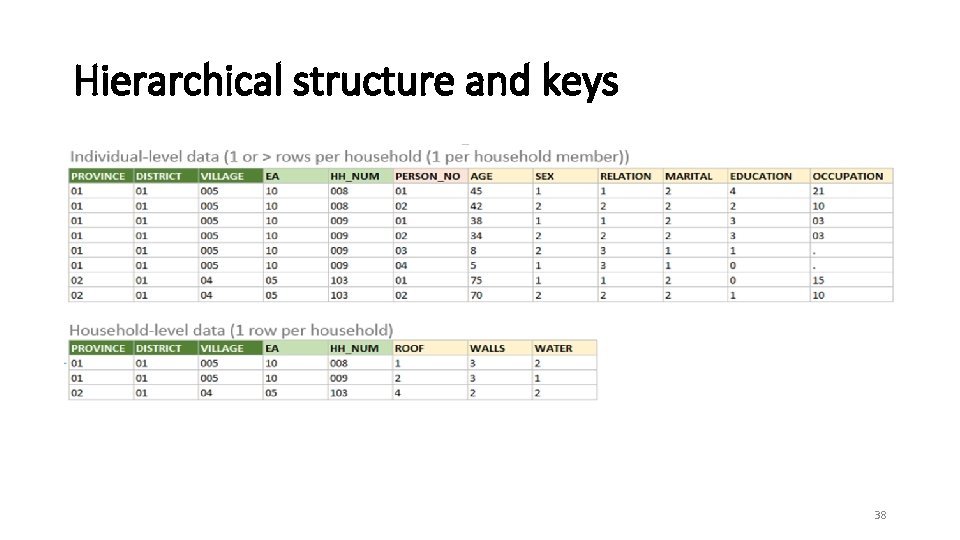
Hierarchical structure of survey datasets • Survey datasets are typically made of multiple related data files • For example, in a household survey, one file may contain: • • Demographic information (1 observation person) Data on education (1 observation person aged 4+) Data on employment (1 observation person aged 15+) Data on births (1 observation per woman aged 12 to 49) Data on dwelling characteristics (1 observation per household) Data on expenditures (1 observation per product/service per household) Etc. • We need “keys” (common variables) to merge these files 37

Hierarchical structure and keys 38

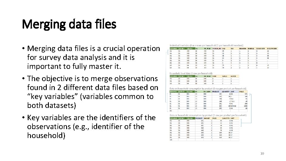
Merging data files • Merging data files is a crucial operation for survey data analysis and it is important to fully master it. • The objective is to merge observations found in 2 different data files based on “key variables” (variables common to both datasets) • Key variables are the identifiers of the observations (e. g. , identifier of the household) 39

Merging data files The relationship between 2 data files can be of different types. The most important for survey data analysts are: • The one-to-one relationships (where one observation from the source file has only one observation in the merged file) • For example: One file contains the demographic information about individuals; the other one contains the employment variables for the sample. • The many-to-one relationships (where multiple observations in the source file correspond to one observation in the merged file) • For example: One file contains the information on individuals (age, sex, etc. ) and the other one contains information on dwelling characteristics. For all members of a same household, there will be one and only one observation about the dwelling characteristics. 40

Merging data files • To merge observations, we need key variables which are variables common to both data files being merged. • In the exercise data files, each household has a unique identifier (variable hhid) and each household member is uniquely identified by a combination of two variables: hhid (which identifies the household) and indid which identifies the person within the household. • In principle, hhid is unique to each household in the householdlevel file, and the combination of hhid and indid is unique to each individual in the person-level data file. • If that is not the case, the merging will not be successful. 41

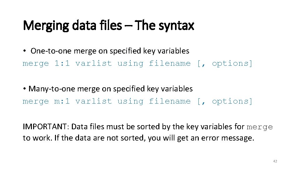
Merging data files – The syntax • One-to-one merge on specified key variables merge 1: 1 varlist using filename [, options] • Many-to-one merge on specified key variables merge m: 1 varlist using filename [, options] IMPORTANT: Data files must be sorted by the key variables for merge to work. If the data are not sorted, you will get an error message. 42

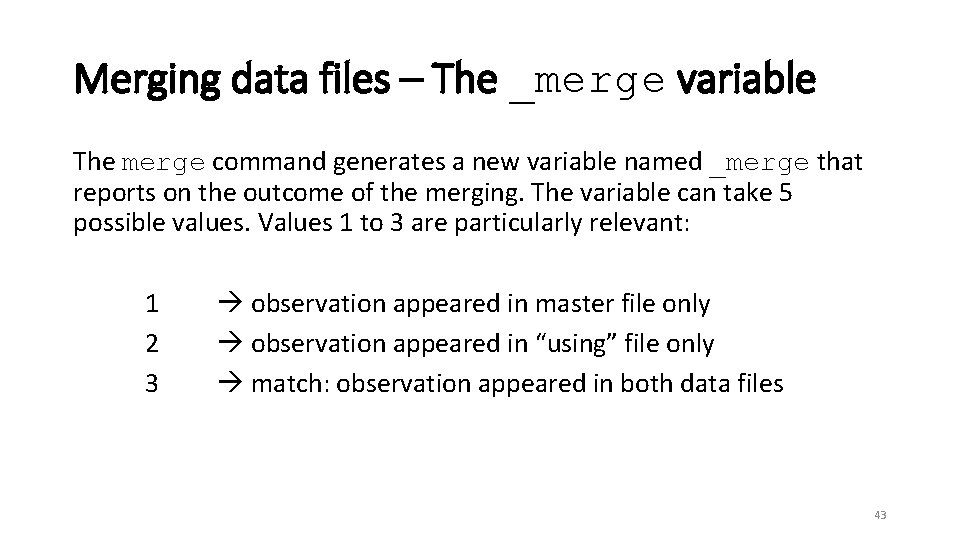
Merging data files – The _merge variable The merge command generates a new variable named _merge that reports on the outcome of the merging. The variable can take 5 possible values. Values 1 to 3 are particularly relevant: 1 observation appeared in master file only 2 observation appeared in “using” file only 3 match: observation appeared in both data files 43

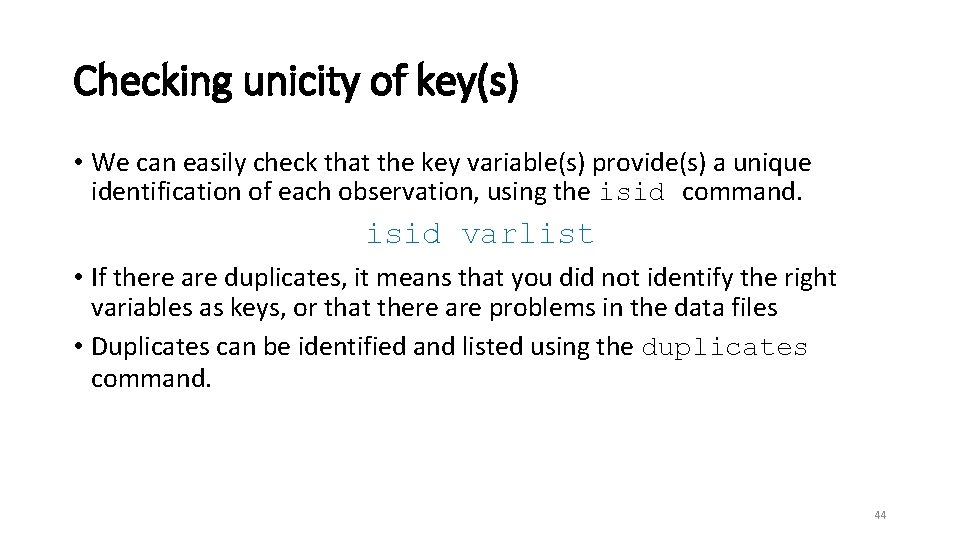
Checking unicity of key(s) • We can easily check that the key variable(s) provide(s) a unique identification of each observation, using the isid command. isid varlist • If there are duplicates, it means that you did not identify the right variables as keys, or that there are problems in the data files • Duplicates can be identified and listed using the duplicates command. 44

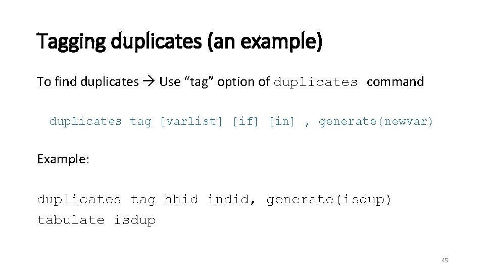
Tagging duplicates (an example) To find duplicates Use “tag” option of duplicates command duplicates tag [varlist] [if] [in] , generate(newvar) Example: duplicates tag hhid indid, generate(isdup) tabulate isdup 45

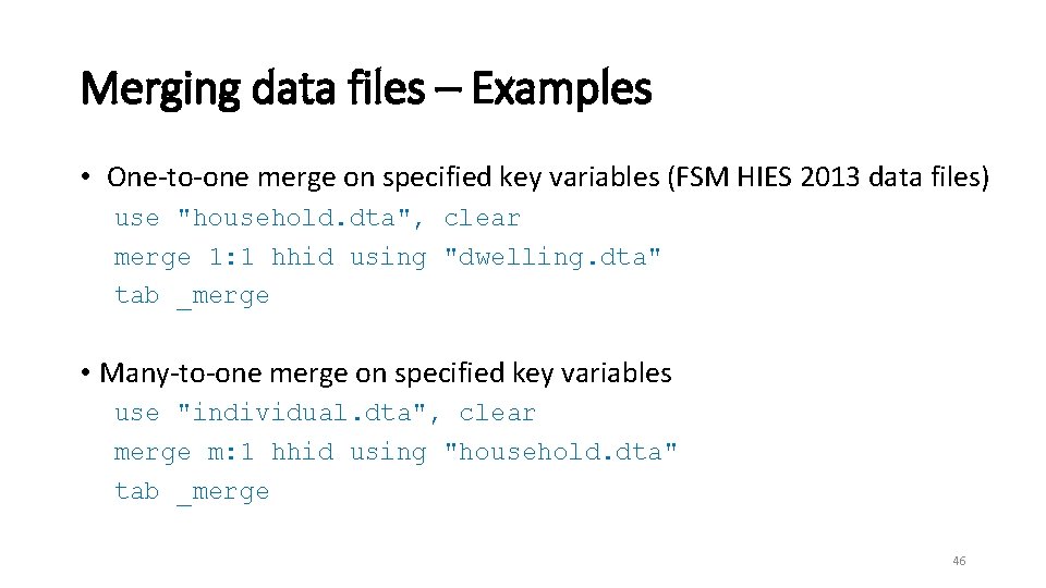
Merging data files – Examples • One-to-one merge on specified key variables (FSM HIES 2013 data files) use "household. dta", clear merge 1: 1 hhid using "dwelling. dta" tab _merge • Many-to-one merge on specified key variables use "individual. dta", clear merge m: 1 hhid using "household. dta" tab _merge 46

Working with variables 47

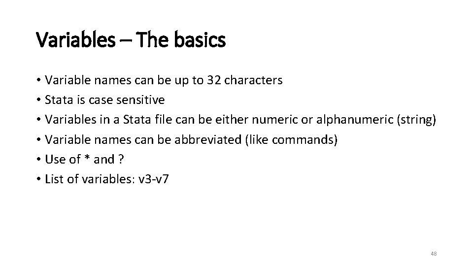
Variables – The basics • Variable names can be up to 32 characters • Stata is case sensitive • Variables in a Stata file can be either numeric or alphanumeric (string) • Variable names can be abbreviated (like commands) • Use of * and ? • List of variables: v 3 -v 7 48

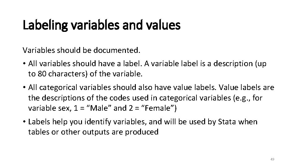
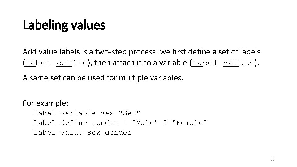
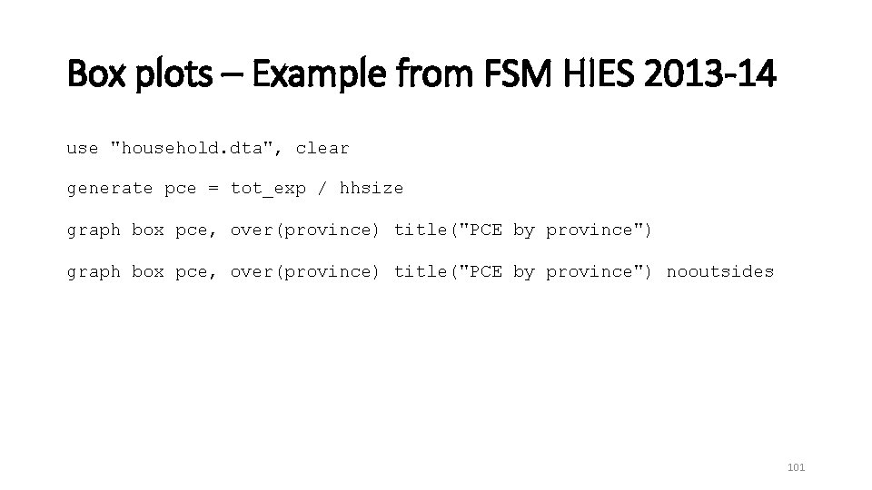
Labeling variables and values Variables should be documented. • All variables should have a label. A variable label is a description (up to 80 characters) of the variable. • All categorical variables should also have value labels. Value labels are the descriptions of the codes used in categorical variables (e. g. , for variable sex, 1 = “Male” and 2 = “Female”) • Labels help you identify variables, and will be used by Stata when tables or other outputs are produced 49

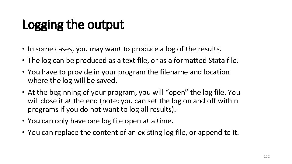
Labeling variables To add a label to a variable: label variable varname ["label"] To change or modify a variable label: same command (will overwrite the existing label) 50

Labeling values Add value labels is a two-step process: we first define a set of labels (label define), then attach it to a variable (label values). A same set can be used for multiple variables. For example: label variable sex "Sex" label define gender 1 "Male" 2 "Female" label value sex gender 51

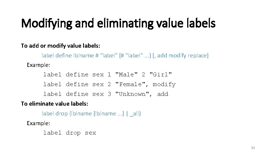
Modifying and eliminating value labels To add or modify value labels: label define lblname # "label" [# "label". . . ] [, add modify replace] Example: label define sex 1 "Male" 2 "Girl" label define sex 2 "Female", modify label define sex 3 "Unknown", add To eliminate value labels: label drop {lblname [lblname. . . ] | _all} Example: label drop sex 52

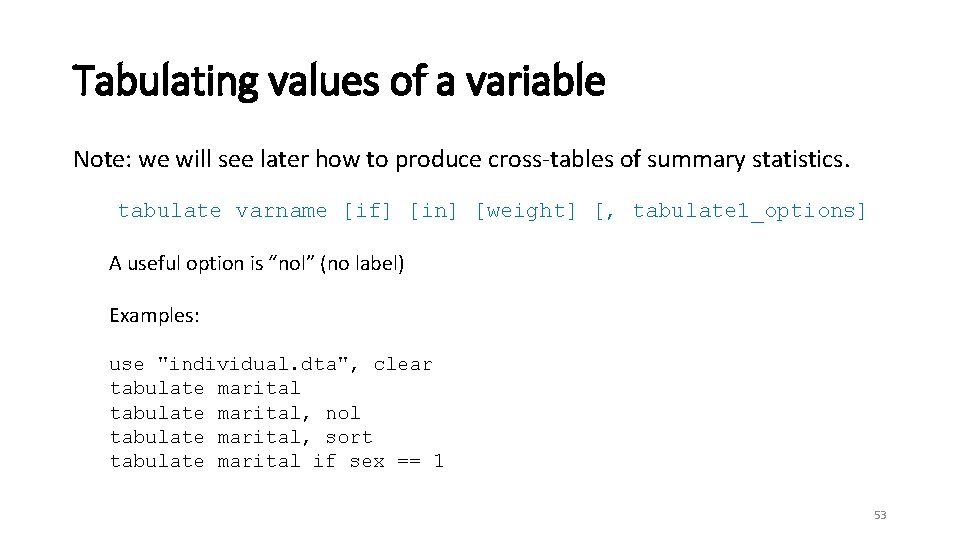
Tabulating values of a variable Note: we will see later how to produce cross-tables of summary statistics. tabulate varname [if] [in] [weight] [, tabulate 1_options] A useful option is “nol” (no label) Examples: use "individual. dta", clear tabulate marital, nol tabulate marital, sort tabulate marital if sex == 1 53

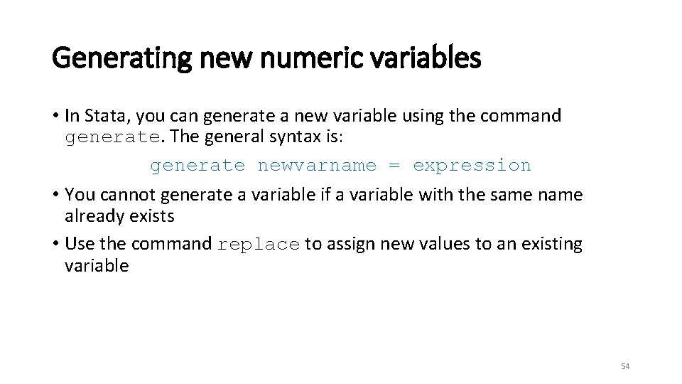
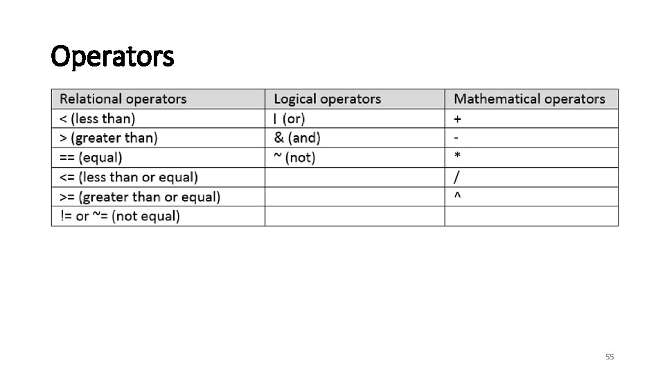
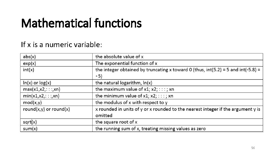
Generating new numeric variables • In Stata, you can generate a new variable using the command generate. The general syntax is: generate newvarname = expression • You cannot generate a variable if a variable with the same name already exists • Use the command replace to assign new values to an existing variable 54

Operators 55

Mathematical functions If x is a numeric variable: 56

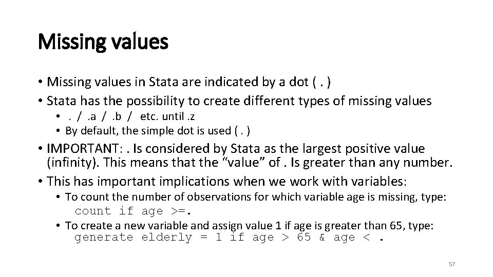
Missing values • Missing values in Stata are indicated by a dot (. ) • Stata has the possibility to create different types of missing values • . / . a / . b / etc. until. z • By default, the simple dot is used (. ) • IMPORTANT: . Is considered by Stata as the largest positive value (infinity). This means that the “value” of. Is greater than any number. • This has important implications when we work with variables: • To count the number of observations for which variable age is missing, type: count if age >=. • To create a new variable and assign value 1 if age is greater than 65, type: generate elderly = 1 if age > 65 & age <. 57

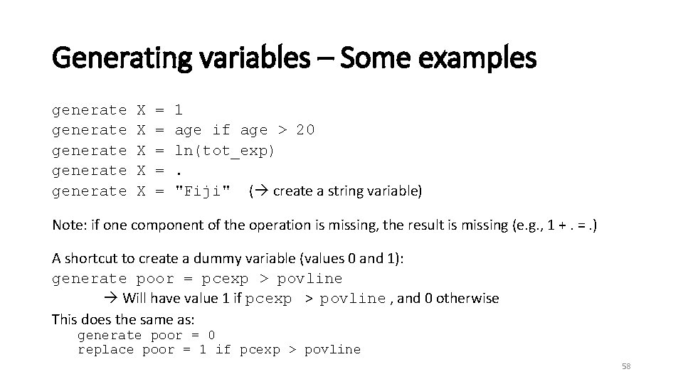
Generating variables – Some examples generate generate X X X = = = 1 age if age > 20 ln(tot_exp). "Fiji" ( create a string variable) Note: if one component of the operation is missing, the result is missing (e. g. , 1 +. =. ) A shortcut to create a dummy variable (values 0 and 1): generate poor = pcexp > povline Will have value 1 if pcexp > povline , and 0 otherwise This does the same as: generate poor = 0 replace poor = 1 if pcexp > povline 58

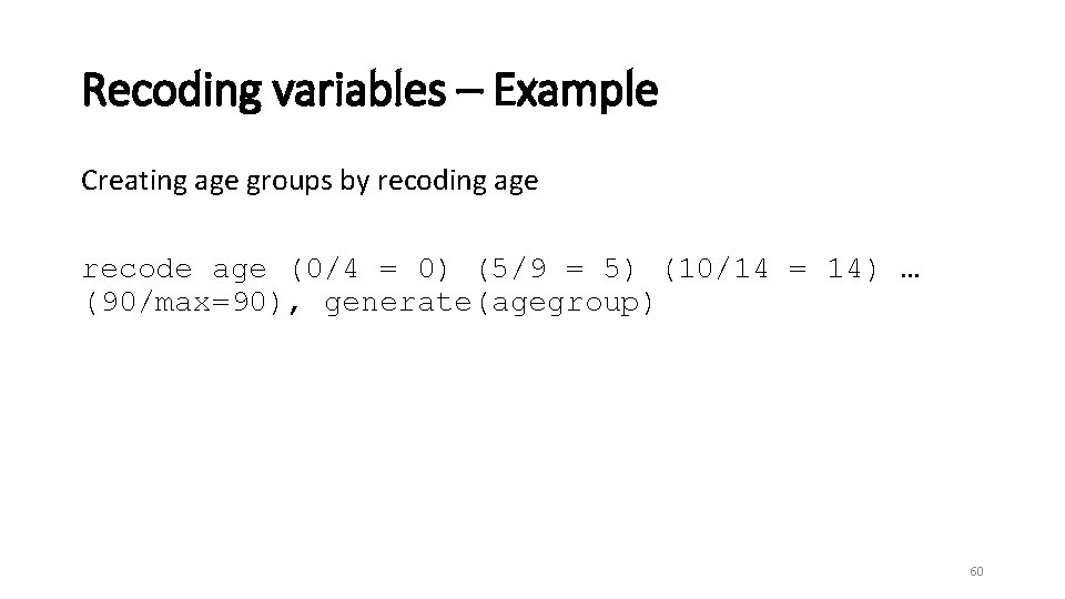
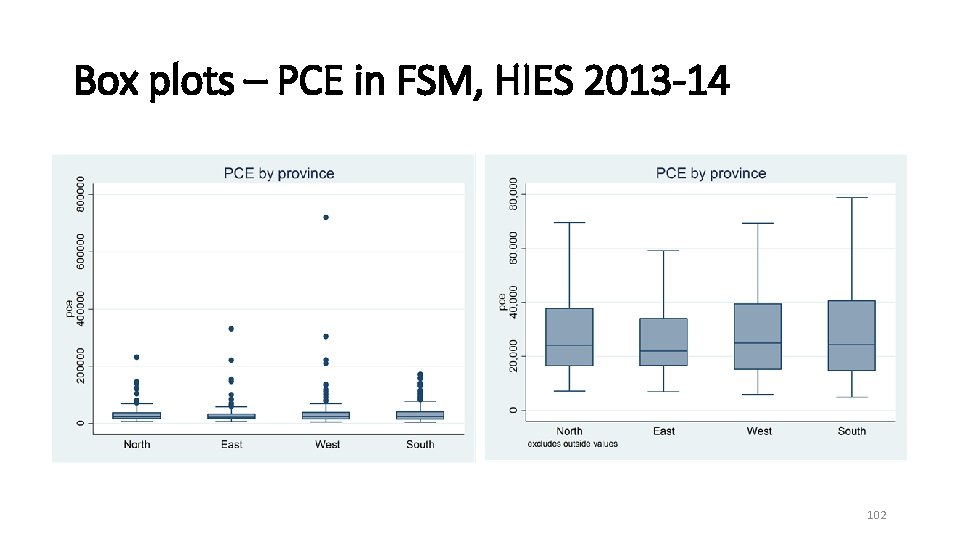
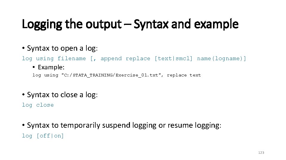
Recoding variables Syntax: recode varlist (rule) [(rule). . . ] [, generate(newvar)] 59

Recoding variables – Example Creating age groups by recoding age recode age (0/4 = 0) (5/9 = 5) (10/14 = 14) … (90/max=90), generate(agegroup) 60

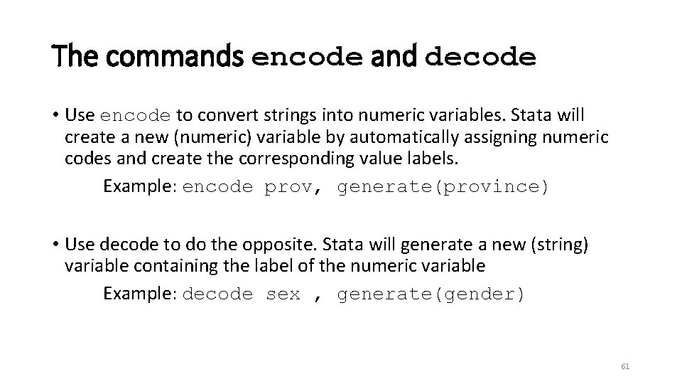
The commands encode and decode • Use encode to convert strings into numeric variables. Stata will create a new (numeric) variable by automatically assigning numeric codes and create the corresponding value labels. Example: encode prov, generate(province) • Use decode to do the opposite. Stata will generate a new (string) variable containing the label of the numeric variable Example: decode sex , generate(gender) 61

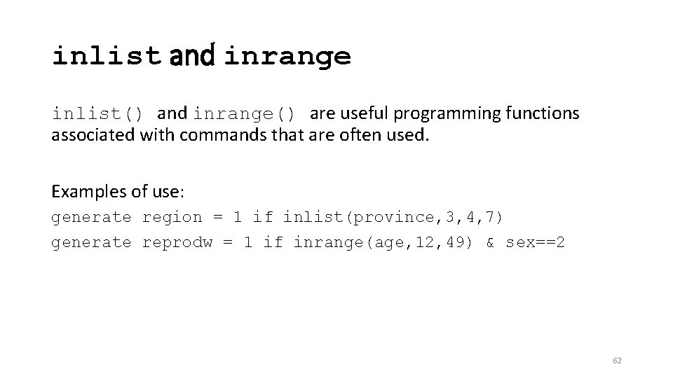
inlist and inrange inlist() and inrange() are useful programming functions associated with commands that are often used. Examples of use: generate region = 1 if inlist(province, 3, 4, 7) generate reprodw = 1 if inrange(age, 12, 49) & sex==2 62

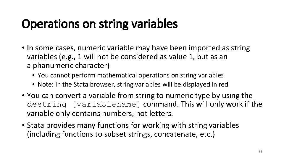
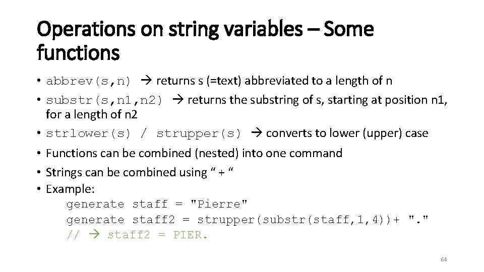
Operations on string variables • In some cases, numeric variable may have been imported as string variables (e. g. , 1 will not be considered as value 1, but as an alphanumeric character) • You cannot perform mathematical operations on string variables • Note: in the Stata browser, string variables will be displayed in red • You can convert a variable from string to numeric type by using the destring [variablename] command. This will only work if the variable only contains numbers, not letters. • Stata provides many functions for working with string variables (including functions to subset strings, concatenate, etc. ) 63

Operations on string variables – Some functions • abbrev(s, n) returns s (=text) abbreviated to a length of n • substr(s, n 1, n 2) returns the substring of s, starting at position n 1, for a length of n 2 • strlower(s) / strupper(s) converts to lower (upper) case • Functions can be combined (nested) into one command • Strings can be combined using “ + “ • Example: generate staff = "Pierre" generate staff 2 = strupper(substr(staff, 1, 4))+ ". " // staff 2 = PIER. 64

Renaming variables rename changes the name of an existing variable Example: rename age_years Stata provides some functions for renaming groups of variables; see help rename group 65

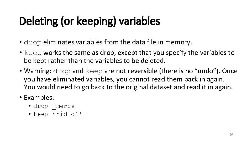
Deleting (or keeping) variables • drop eliminates variables from the data file in memory. • keep works the same as drop, except that you specify the variables to be kept rather than the variables to be deleted. • Warning: drop and keep are not reversible (there is no “undo”). Once you have eliminated variables, you cannot read them back in again. You would need to go back to the original dataset and read it in again. • Examples: • drop _merge • keep hhid q 1* 66

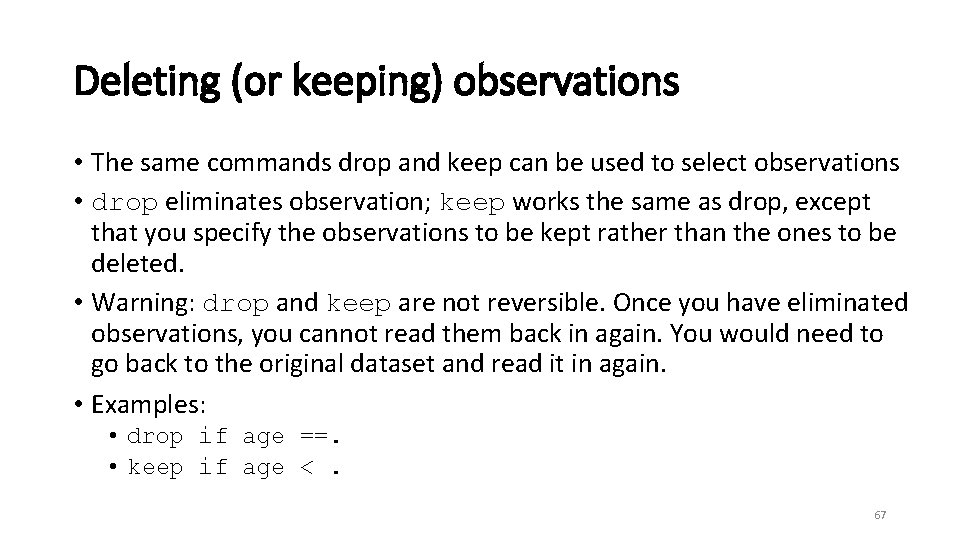
Deleting (or keeping) observations • The same commands drop and keep can be used to select observations • drop eliminates observation; keep works the same as drop, except that you specify the observations to be kept rather than the ones to be deleted. • Warning: drop and keep are not reversible. Once you have eliminated observations, you cannot read them back in again. You would need to go back to the original dataset and read it in again. • Examples: • drop if age ==. • keep if age <. 67

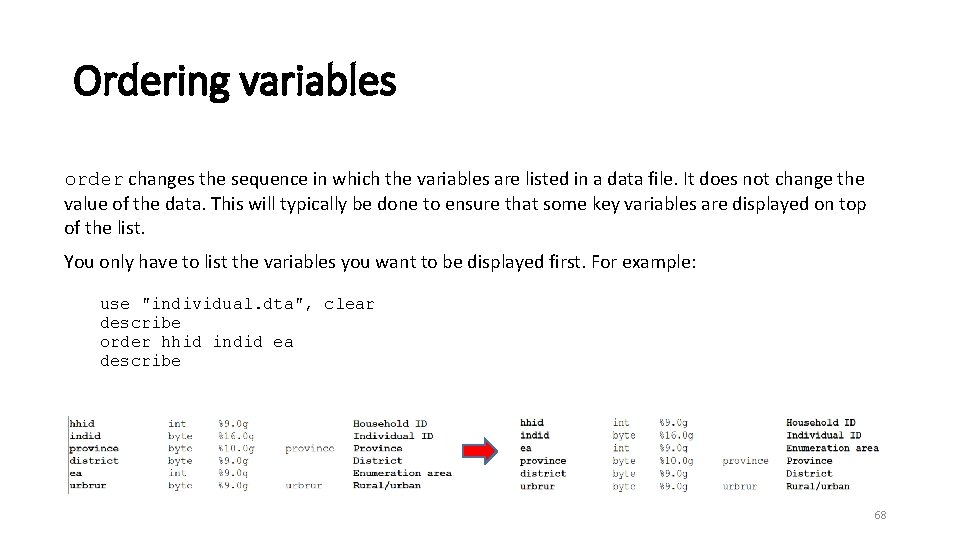
Ordering variables order changes the sequence in which the variables are listed in a data file. It does not change the value of the data. This will typically be done to ensure that some key variables are displayed on top of the list. You only have to list the variables you want to be displayed first. For example: use "individual. dta", clear describe order hhid indid ea describe 68

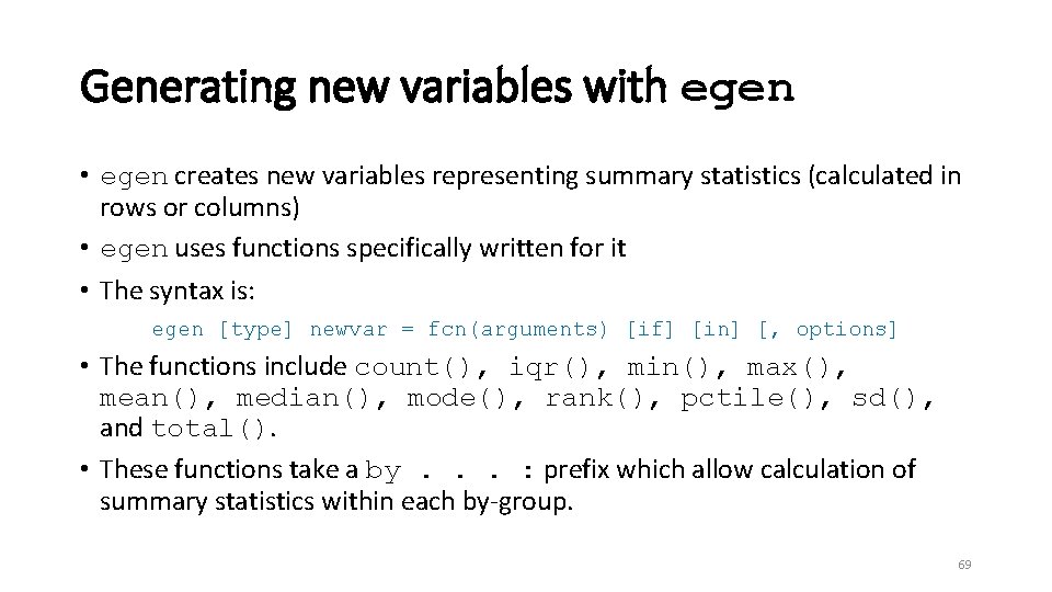
Generating new variables with egen • egen creates new variables representing summary statistics (calculated in rows or columns) • egen uses functions specifically written for it • The syntax is: egen [type] newvar = fcn(arguments) [if] [in] [, options] • The functions include count(), iqr(), min(), max(), mean(), median(), mode(), rank(), pctile(), sd(), and total(). • These functions take a by. . . : prefix which allow calculation of summary statistics within each by-group. 69

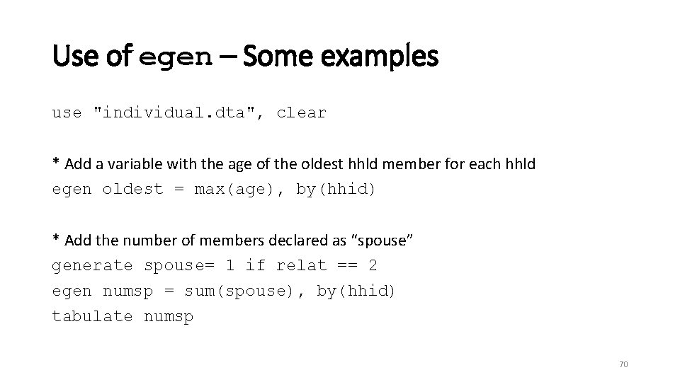
Use of egen – Some examples use "individual. dta", clear * Add a variable with the age of the oldest hhld member for each hhld egen oldest = max(age), by(hhid) * Add the number of members declared as “spouse” generate spouse= 1 if relat == 2 egen numsp = sum(spouse), by(hhid) tabulate numsp 70

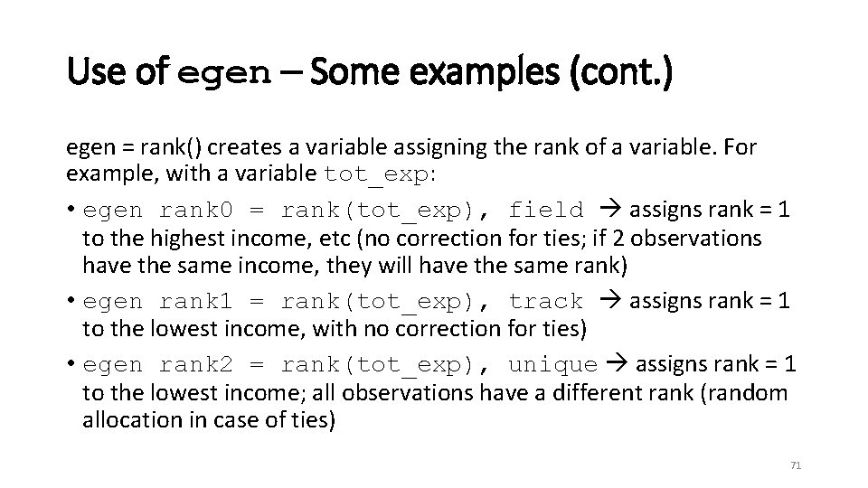
Use of egen – Some examples (cont. ) egen = rank() creates a variable assigning the rank of a variable. For example, with a variable tot_exp: • egen rank 0 = rank(tot_exp), field assigns rank = 1 to the highest income, etc (no correction for ties; if 2 observations have the same income, they will have the same rank) • egen rank 1 = rank(tot_exp), track assigns rank = 1 to the lowest income, with no correction for ties) • egen rank 2 = rank(tot_exp), unique assigns rank = 1 to the lowest income; all observations have a different rank (random allocation in case of ties) 71

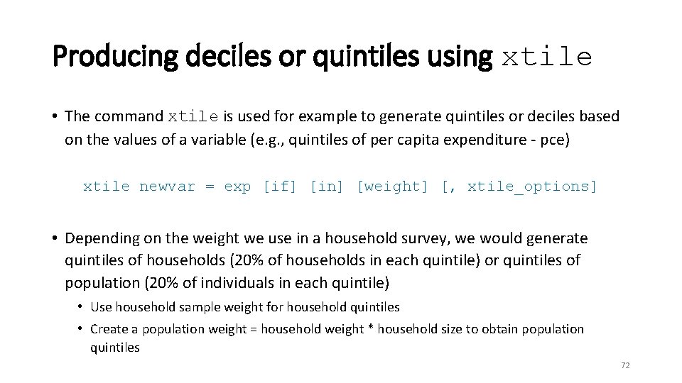
Producing deciles or quintiles using xtile • The command xtile is used for example to generate quintiles or deciles based on the values of a variable (e. g. , quintiles of per capita expenditure - pce) xtile newvar = exp [if] [in] [weight] [, xtile_options] • Depending on the weight we use in a household survey, we would generate quintiles of households (20% of households in each quintile) or quintiles of population (20% of individuals in each quintile) • Use household sample weight for household quintiles • Create a population weight = household weight * household size to obtain population quintiles 72

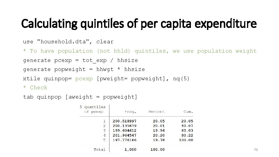
Calculating quintiles of per capita expenditure use "household. dta", clear * To have population (not hhld) quintiles, we use population weight generate pcexp = tot_exp / hhsize generate popweight = hhwgt * hhsize xtile quinpop= pcexp [pweight= popweight], nq(5) * Check tab quinpop [aweight = popweight] 73

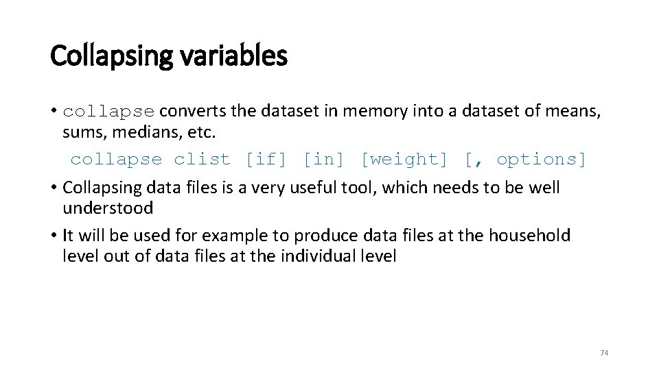
Collapsing variables • collapse converts the dataset in memory into a dataset of means, sums, medians, etc. collapse clist [if] [in] [weight] [, options] • Collapsing data files is a very useful tool, which needs to be well understood • It will be used for example to produce data files at the household level out of data files at the individual level 74

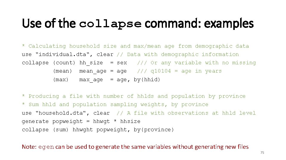
Use of the collapse command: examples * Calculating household size and max/mean age from demographic data use "individual. dta", clear // Data with demographic information collapse (count) hh_size = sex /// Or any variable with no missing (mean) mean_age = age /// q 10104 = age in years (max) max_age = age, by(hhid) * Producing a file with number of hhlds and population by province * Sum hhld and population sampling weights, by province use "household. dta", clear // A file with observations at hhld level generate popweight = hhwgt * hhsize collapse (sum) hhwght popweight, by(province) Note: egen can be used to generate the same variables without generating new files 75

Use of duplicates drop One way to keep only one observation per group (e. g. , per household) is to use collapse. Another way is to remove all duplicates of the key variables using the duplicates drop command. duplicates drop varlist [if] [in], force 76

Generating dummy variables • Dummy variables are variables with values 0 (false) and 1 (true). We already saw how to generate a dummy variable using the generate command, e. g. • The long way: generate male = 0 replace male = 1 if sex == 1 • The short way: generate male = sex==1 • When you have multiple categories, this method is tedious. You can use the tabulate command instead. For example: tabulate province, gen(prov) This will create dummy variables prov 1, prov 2, prov 3, …, prov. N (one dummy for each province) • One additional option is to use the xi command (see slides on regression). 77

Producing tables 78

Tabulation • We saw in a previous slide that frequency tables can easily be produced using the tabulate command (see also tab 1 and tab 2). • For producing multi-dimension tables with summary statistics, we will use the table commands. • Stata also provides the command tabstat for producing tables with summary statistics for a series of numeric variables. • A user-contributed package (ado file) named tabout complements the Stata tabulation commands. 79

A note on copy/pasting tables • To copy and paste tables from the Stata results window, use the copy table option, not copy. The formatting of the table will then be preserved, and cells will be properly distinguished when pasting to Excel. 80

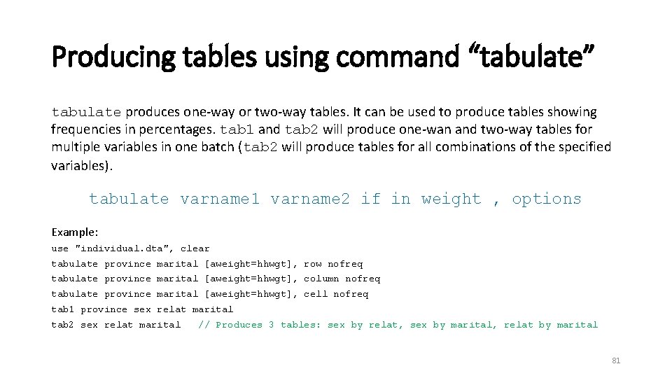
Producing tables using command “tabulate” tabulate produces one-way or two-way tables. It can be used to produce tables showing frequencies in percentages. tab 1 and tab 2 will produce one-wan and two-way tables for multiple variables in one batch (tab 2 will produce tables for all combinations of the specified variables). tabulate varname 1 varname 2 if in weight , options Example: use "individual. dta", clear tabulate province marital [aweight=hhwgt], row nofreq tabulate province marital [aweight=hhwgt], column nofreq tabulate province marital [aweight=hhwgt], cell nofreq tab 1 province sex relat marital tab 2 sex relat marital // Produces 3 tables: sex by relat, sex by marital, relat by marital 81

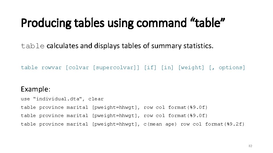
Producing tables using command “table” table calculates and displays tables of summary statistics. table rowvar [colvar [supercolvar]] [if] [in] [weight] [, options] Example: use "individual. dta", clear table province marital [pweight=hhwgt], row col format(%9. 0 f) table province marital [pweight=hhwgt], c(mean age) row col format(%9. 2 f) 82

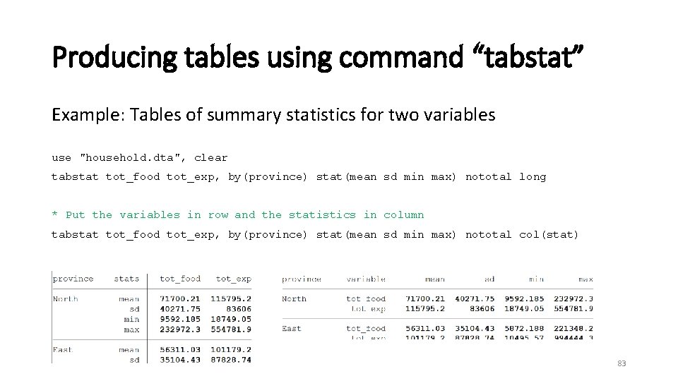
Producing tables using command “tabstat” Example: Tables of summary statistics for two variables use "household. dta", clear tabstat tot_food tot_exp, by(province) stat(mean sd min max) nototal long * Put the variables in row and the statistics in column tabstat tot_food tot_exp, by(province) stat(mean sd min max) nototal col(stat) 83

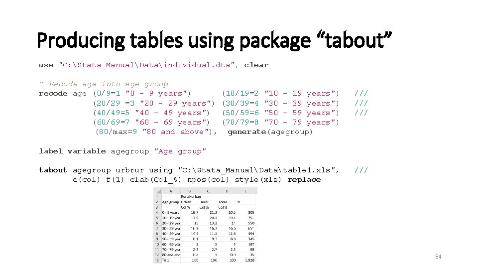
Producing tables using package “tabout” use "C: Stata_ManualDataindividual. dta", clear * Recode age into age group recode age (0/9=1 "0 - 9 years") (20/29 =3 "20 - 29 years") (40/49=5 "40 - 49 years") (60/69=7 "60 - 69 years") (80/max=9 "80 and above"), (10/19=2 "10 - 19 years") (30/39=4 "30 - 39 years") (50/59=6 "50 - 59 years") (70/79=8 "70 - 79 years") generate(agegroup) /// /// tabout agegroup urbrur using "C: Stata_ManualDatatable 1. xls", c(col) f(1) clab(Col_%) npos(col) style(xls) replace /// label variable agegroup "Age group" 84

Producing graphs 85

Graphs Stata has powerful graph capabilities. Producing simple charts is very easy. But Stata offers many options that allows you to generate complex ones, and to customize about every aspect of your charts. A full manual is dedicated to it. Tip: Use the menu-driven tools, which will produce the code for you. We only show here some basic, common commands. Once you master these commands, read the Stata manual for more. Or visit Stata’s online “Visual overview for creating graphs” at: http: //www. stata. com/support/faqs/graphics/gph/stata-graphs/ 86

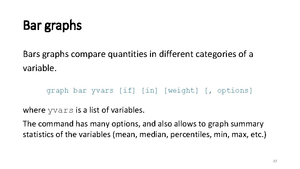
Bar graphs Bars graphs compare quantities in different categories of a variable. graph bar yvars [if] [in] [weight] [, options] where yvars is a list of variables. The command has many options, and also allows to graph summary statistics of the variables (mean, median, percentiles, min, max, etc. ) 87

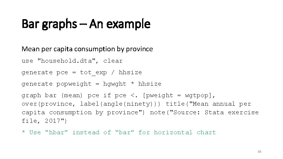
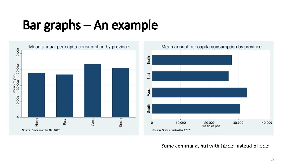
Bar graphs – An example Mean per capita consumption by province use "household. dta", clear generate pce = tot_exp / hhsize generate popweight = hgwght * hhsize graph bar (mean) pce if pce <. [pweight = wgtpop], over(province, label(angle(ninety))) title("Mean annual per capita consumption by province") note("Source: Stata exercise file, 2017") * Use “hbar” instead of “bar” for horizontal chart 88

Bar graphs – An example Same command, but with hbar instead of bar 89

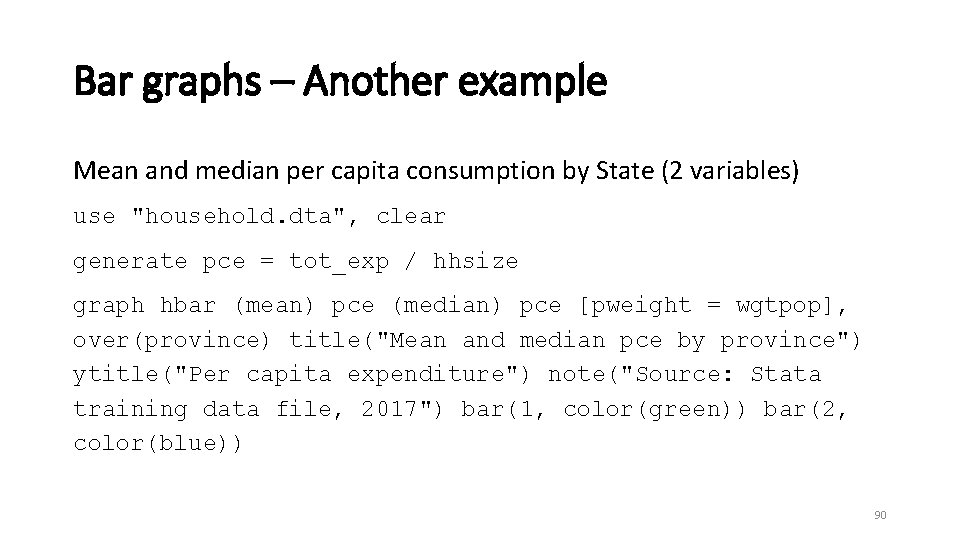
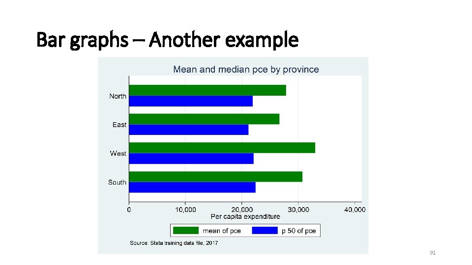
Bar graphs – Another example Mean and median per capita consumption by State (2 variables) use "household. dta", clear generate pce = tot_exp / hhsize graph hbar (mean) pce (median) pce [pweight = wgtpop], over(province) title("Mean and median pce by province") ytitle("Per capita expenditure") note("Source: Stata training data file, 2017") bar(1, color(green)) bar(2, color(blue)) 90

Bar graphs – Another example 91

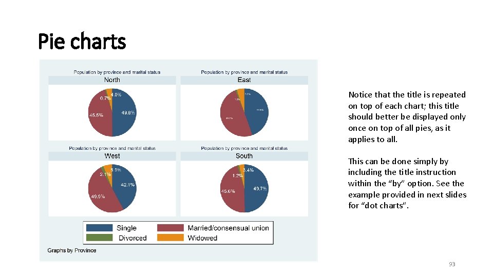
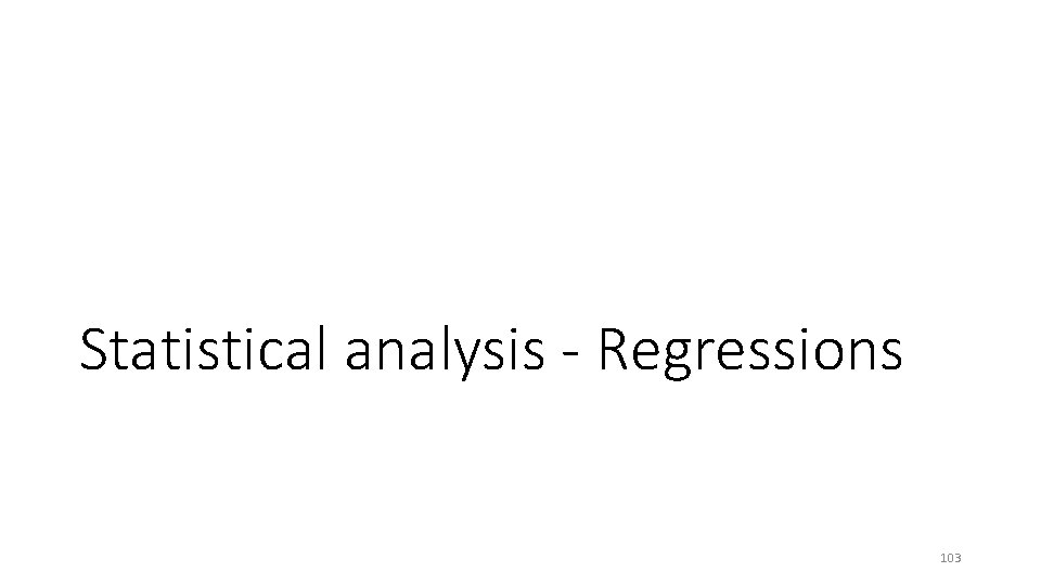
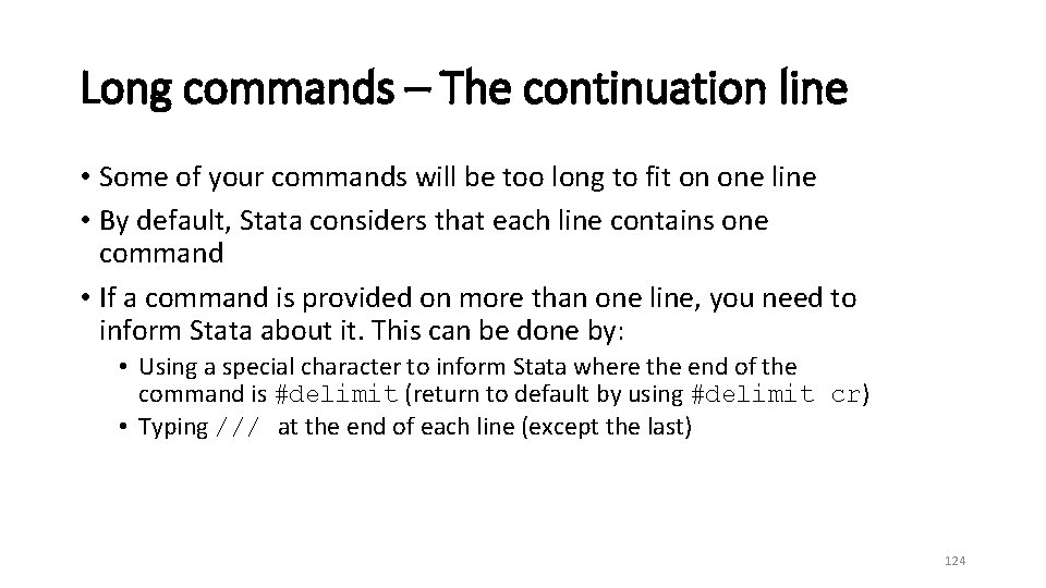
Pie charts • Syntax: graph pie varlist [if] [in] [weight] [, options] • Example: use "individual. dta", clear graph pie [pweight = hhwgt], over(marital) plabel(_all percent, color(white) format(%9. 1 f)) cw by(, legend(on)) by(province, title(Population by province and marital status)) 92

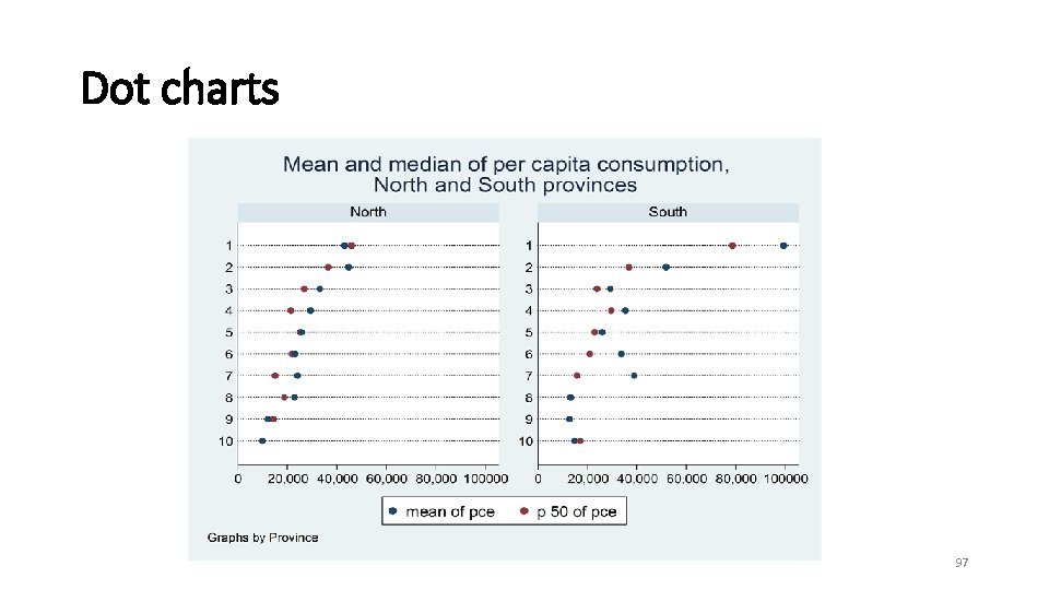
Pie charts Notice that the title is repeated on top of each chart; this title should better be displayed only once on top of all pies, as it applies to all. This can be done simply by including the title instruction within the “by” option. See the example provided in next slides for “dot charts”. 93

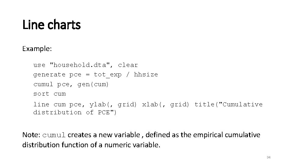
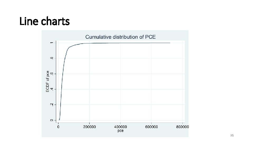
Line charts Example: use "household. dta", clear generate pce = tot_exp / hhsize cumul pce, gen(cum) sort cum line cum pce, ylab(, grid) xlab(, grid) title("Cumulative distribution of PCE") Note: cumul creates a new variable , defined as the empirical cumulative distribution function of a numeric variable. 94

Line charts 95

Dot charts use "household. dta", clear generate pce = tot_exp / hhsize recode hhsize (10/max=10), generate(hhsize 2) keep if province == 1 | province == 4 // We keep only two provinces graph dot (mean) pce (p 50) pce [pweight=wgtpop], over(hhsize 2) by(province, title("Mean and median of per capita consumption, " "North and South provinces")) // The title is within the ‘by’ option 96

Dot charts 97

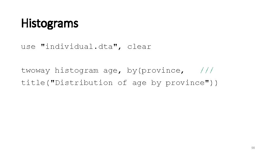
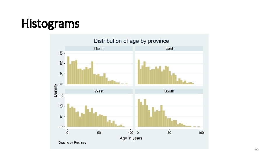
Histograms use "individual. dta", clear twoway histogram age, by(province, /// title("Distribution of age by province")) 98

Histograms 99

Box plots • The box plot (a. k. a. box and whisker diagram) is a standardized way of displaying the distribution of data based on the five number summary: minimum, first quartile, median, third quartile, and maximum. • In the simplest box plot the central rectangle spans the first quartile to the third quartile (the interquartile range or IQR). • A segment inside the rectangle shows the median and "whiskers" above and below the box show the locations of the minimum and maximum. 100

Box plots – Example from FSM HIES 2013 14 use "household. dta", clear generate pce = tot_exp / hhsize graph box pce, over(province) title("PCE by province") nooutsides 101

Box plots – PCE in FSM, HIES 2013 14 102

Statistical analysis - Regressions 103

Regressions in Stata • Stata provides commands for running many types of regressions (linear, non-linear, logistic, probit, quantile, etc. ) • The most common types are the linear and the logistic models. • The linear model used to predict the value of a continuous variable based on the value of one or more independent variables • The logistic model used to predict the value of a binary variable (e. g. , poor / non-poor) or a categorical variable with more than 2 categories (multinomial regression) • Some specific commands allow taking complex survey designs into consideration (command svyreg). 104

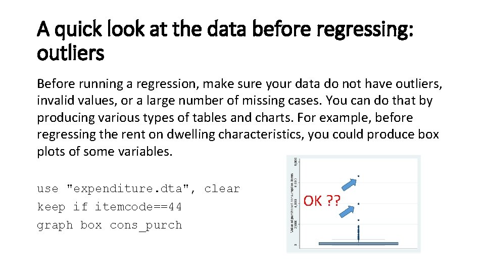
A quick look at the data before regressing: outliers Before running a regression, make sure your data do not have outliers, invalid values, or a large number of missing cases. You can do that by producing various types of tables and charts. For example, before regressing the rent on dwelling characteristics, you could produce box plots of some variables. use "expenditure. dta", clear keep if itemcode==44 graph box cons_purch OK ? ?

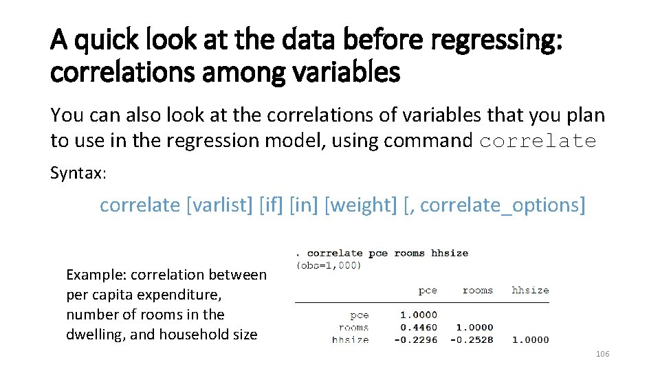
A quick look at the data before regressing: correlations among variables You can also look at the correlations of variables that you plan to use in the regression model, using command correlate Syntax: correlate [varlist] [if] [in] [weight] [, correlate_options] Example: correlation between per capita expenditure, number of rooms in the dwelling, and household size 106

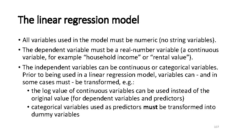
The linear regression model • All variables used in the model must be numeric (no string variables). • The dependent variable must be a real-number variable (a continuous variable, for example “household income” or “rental value”). • The independent variables can be continuous or categorical variables. Prior to being used in a linear regression model, variables can - and in some cases must - be transformed, e. g. : • the log value of continuous variables can be used instead of the original value (for dependent variables and predictors) • categorical variables used as predictors must be transformed into dummy variables 107

Linear regression: regress, predict • regress performs ordinary least-squares linear regression. • The syntax is: regress depvar [indepvars] [if] [in] [weight] [, options] • Once a model has been fit using the regress command, it can be applied to data to predict values of the dependent variable using the predict command. This command will make prediction using the latest regression model run by Stata. For a single-equation model, the syntax is: predict [type] newvar [if] [in] [, options] 108

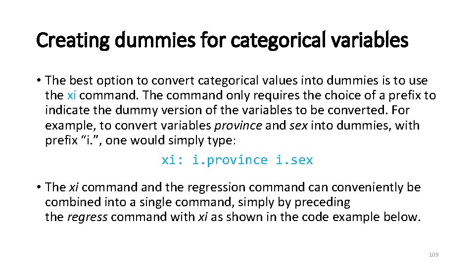
Creating dummies for categorical variables • The best option to convert categorical values into dummies is to use the xi command. The command only requires the choice of a prefix to indicate the dummy version of the variables to be converted. For example, to convert variables province and sex into dummies, with prefix “i. ”, one would simply type: xi: i. province i. sex • The xi command the regression command can conveniently be combined into a single command, simply by preceding the regress command with xi as shown in the code example below. 109

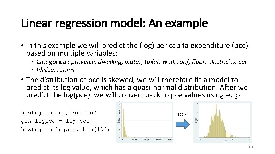
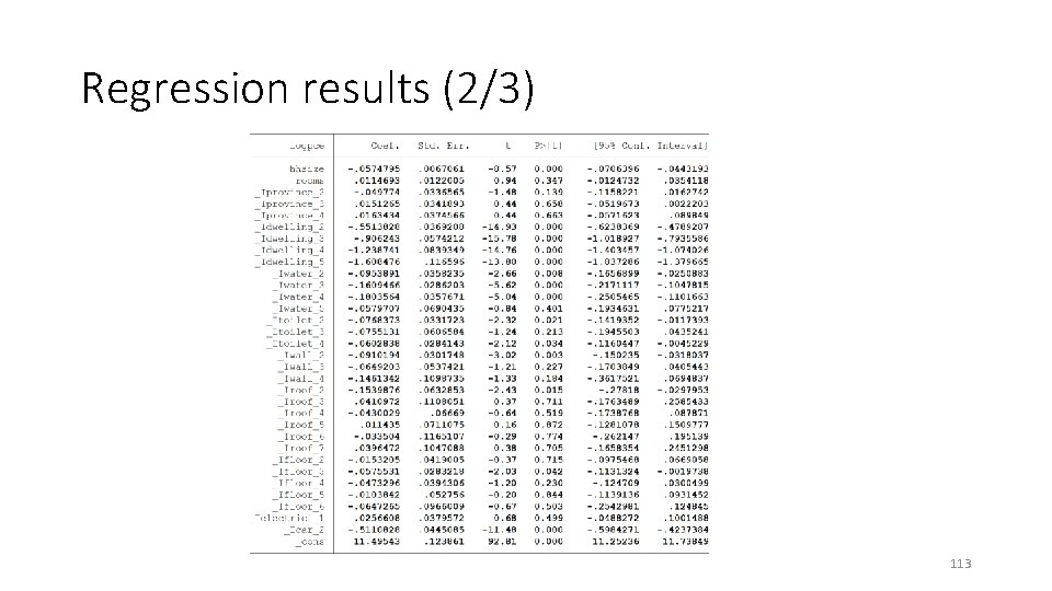
Linear regression model: An example • In this example we will predict the (log) per capita expenditure (pce) based on multiple variables: • Categorical: province, dwelling, water, toilet, wall, roof, floor, electricity, car • hhsize, rooms • The distribution of pce is skewed; we will therefore fit a model to predict its log value, which has a quasi-normal distribution. After we predict the log(pce), we will convert back to pce values using exp. histogram pce, bin(100) gen logpce = log(pce) histogram logpce, bin(100) LOG 110

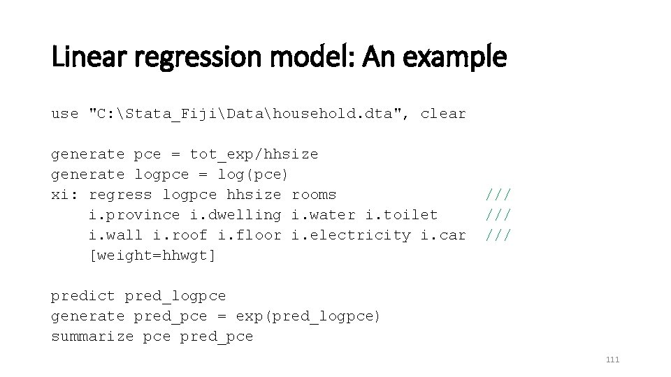
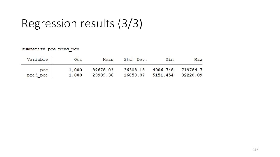
Linear regression model: An example use "C: Stata_FijiDatahousehold. dta", clear generate pce = tot_exp/hhsize generate logpce = log(pce) xi: regress logpce hhsize rooms i. province i. dwelling i. water i. toilet i. wall i. roof i. floor i. electricity i. car [weight=hhwgt] /// /// predict pred_logpce generate pred_pce = exp(pred_logpce) summarize pce pred_pce 111

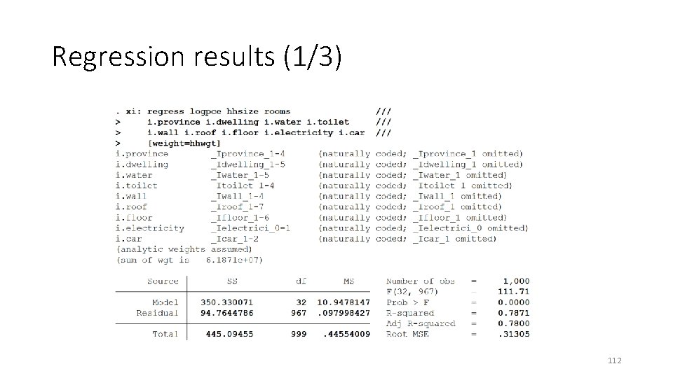
Regression results (1/3) 112

Regression results (2/3) 113

Regression results (3/3) 114

Logistic regression, a. k. a. logit model • Logistic regression predicts dichotomous variables, i. e. the dependent variable is binary (true/false, yes/no, poor/non-poor, etc. ) • Alternative: probit regression • Two commands in Stata: logit and logistic (same, except that logistic displays estimates as odds ratios) • Syntax (see Stata help for detail on options): logit depvar [indepvars] [if] [in] [weight] [, options] or logistic depvar indepvars [if] [in] [weight] [, options] 115

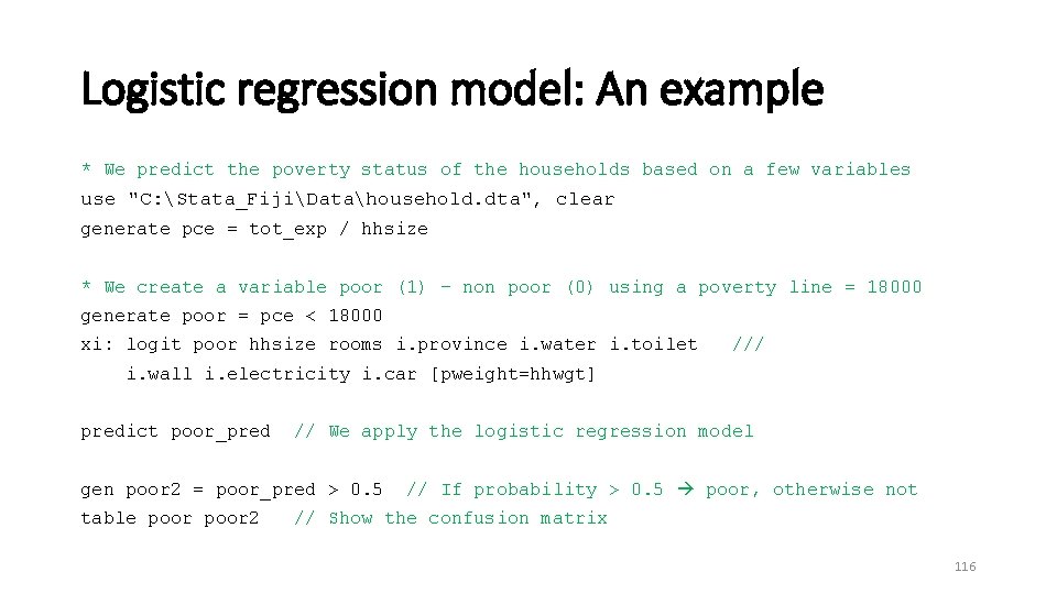
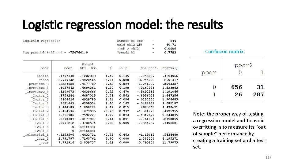
Logistic regression model: An example * We predict the poverty status of the households based on a few variables use "C: Stata_FijiDatahousehold. dta", clear generate pce = tot_exp / hhsize * We create a variable poor (1) – non poor (0) using a poverty line = 18000 generate poor = pce < 18000 xi: logit poor hhsize rooms i. province i. water i. toilet /// i. wall i. electricity i. car [pweight=hhwgt] predict poor_pred // We apply the logistic regression model gen poor 2 = poor_pred > 0. 5 table poor 2 // If probability > 0. 5 poor, otherwise not // Show the confusion matrix 116

Logistic regression model: the results Confusion matrix: Note: the proper way of testing a regression model and to avoid overfitting is to measure its “out of sample” performance by creating a training set and a test set. 117

Programming in Stata 118

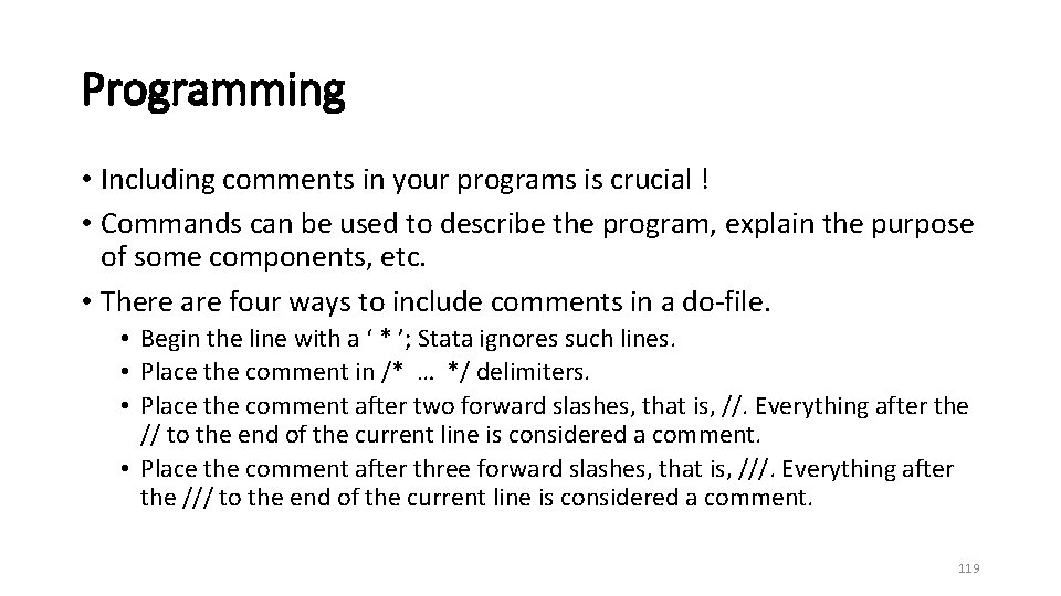
Programming • Including comments in your programs is crucial ! • Commands can be used to describe the program, explain the purpose of some components, etc. • There are four ways to include comments in a do-file. • Begin the line with a ‘ * ’; Stata ignores such lines. • Place the comment in /* … */ delimiters. • Place the comment after two forward slashes, that is, //. Everything after the // to the end of the current line is considered a comment. • Place the comment after three forward slashes, that is, ///. Everything after the /// to the end of the current line is considered a comment. 119

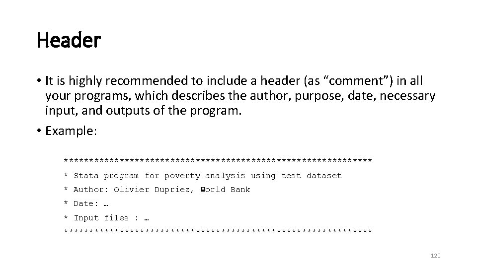
Header • It is highly recommended to include a header (as “comment”) in all your programs, which describes the author, purpose, date, necessary input, and outputs of the program. • Example: ******************************* * Stata program for poverty analysis using test dataset * Author: Olivier Dupriez, World Bank * Date: … * Input files : … ******************************* 120

version, and set more off • The first commands that you will include in your programs will often be version and set more off • version indicates which version of Stata you are writing the program for (Stata evolves, and some commands can change) • set more off is a parameter that controls the display of the results • Example: version 14 set more off 121

Logging the output • In some cases, you may want to produce a log of the results. • The log can be produced as a text file, or as a formatted Stata file. • You have to provide in your program the filename and location where the log will be saved. • At the beginning of your program, you will “open” the log file. You will close it at the end (note: you can set the log on and off within programs if you do not want to log all results). • You can only have one log file open at a time. • You can replace the content of an existing log file, or append to it. 122

Logging the output – Syntax and example • Syntax to open a log: log using filename [, append replace [text|smcl] name(logname)] • Example: log using "C: /STATA_TRAINING/Exercise_01. txt", replace text • Syntax to close a log: log close • Syntax to temporarily suspend logging or resume logging: log [off|on] 123

Long commands – The continuation line • Some of your commands will be too long to fit on one line • By default, Stata considers that each line contains one command • If a command is provided on more than one line, you need to inform Stata about it. This can be done by: • Using a special character to inform Stata where the end of the command is #delimit (return to default by using #delimit cr) • Typing /// at the end of each line (except the last) 124

Long commands – Example #delimit ; recode province (17=13)(5=14)(11=15)(16=16)(7=17) (12=18)(3=1)(6=2)(4=3)(2=4)(14=5)(13=6)(10=7)(1=8)(8=9) (15=11)(9=12), gen(prov) ; #delimit cr OR recode province (17=13)(5=14)(11=15)(16=16)(7=17) /// (12=18)(3=1)(6=2)(4=3)(2=4)(14=5)(13=6)(10=7)(1=8)(8=9) /// (15=11)(9=12), gen(prov) 125

Record number and number of records • Stata has two macro variables that you can use any time in your programs • One is named _N and indicates the total number of observations in the file • The other one indicates the sequential number of each observation in the data file and is named _n 126

Macros • In many Stata programs, you will make use of macro variables. These are variables that are not saved in data files, but are available for use during the execution of your programs. • Macros can be local (in which case they only exist within a specific do file) or global (in which case they can be used across programs). • You create a macro variable simply by declaring its type and giving it a value (numeric or string), e. g. , • local i = 1 • global myfolder = "C: Stata_Fiji" 127

Macros • Once a macro has been created and contains some value or text, you can use it in your programs. • To refer to a local variables ina program, put the name of the macro between quotes as follows `macroname’. For global macros, put the character $ before the name (e. g. , $macroname) • Example: local i = 10 display "The value of my local macro is " `i’ global myfolder = "C: Stata_Fiji" display "The content of my global macro is " $myfolder 128

Temporary files • In some programs, you may want to generate data files that are needed only for the execution of that program. You can create such temporary files using the tempfile command. Temporary files are automatically erased at completion of the program’s execution. • You can create multiple temporary files in a program. • You create them by giving them a name before putting content in them. Example: to create 2 temporary files named t 0 and t 1, type: tempfile t 0 t 1 • The command tempfile can be put anywhere in your program. • To refer to a tempfile, enclose its name into single quotes (like local macros). Example: save `t 0’, replace 129

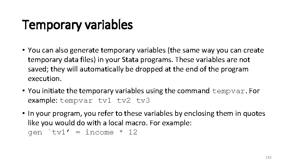
Temporary variables • You can also generate temporary variables (the same way you can create temporary data files) in your Stata programs. These variables are not saved; they will automatically be dropped at the end of the program execution. • You initiate the temporary variables using the command tempvar. For example: tempvar tv 1 tv 2 tv 3 • In your program, you refer to these variables by enclosing them in quotes like you would do with a local macro. For example: gen `tv 1’ = income * 12 130

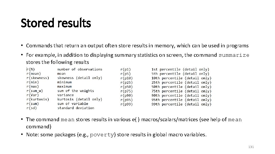
Stored results • Commands that return an output often store results in memory, which can be used in programs • For example, in addition to displaying summary statistics on screen, the command summarize stores the following results • The command mean stores results in various e( ) macros/scalars/matrices (see help of mean command) • Note: some packages (e. g. , poverty) store results in global macro variables. 131

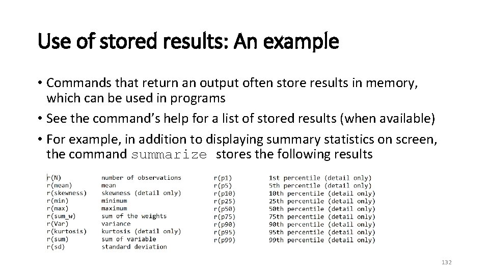
Use of stored results: An example • Commands that return an output often store results in memory, which can be used in programs • See the command’s help for a list of stored results (when available) • For example, in addition to displaying summary statistics on screen, the command summarize stores the following results 132

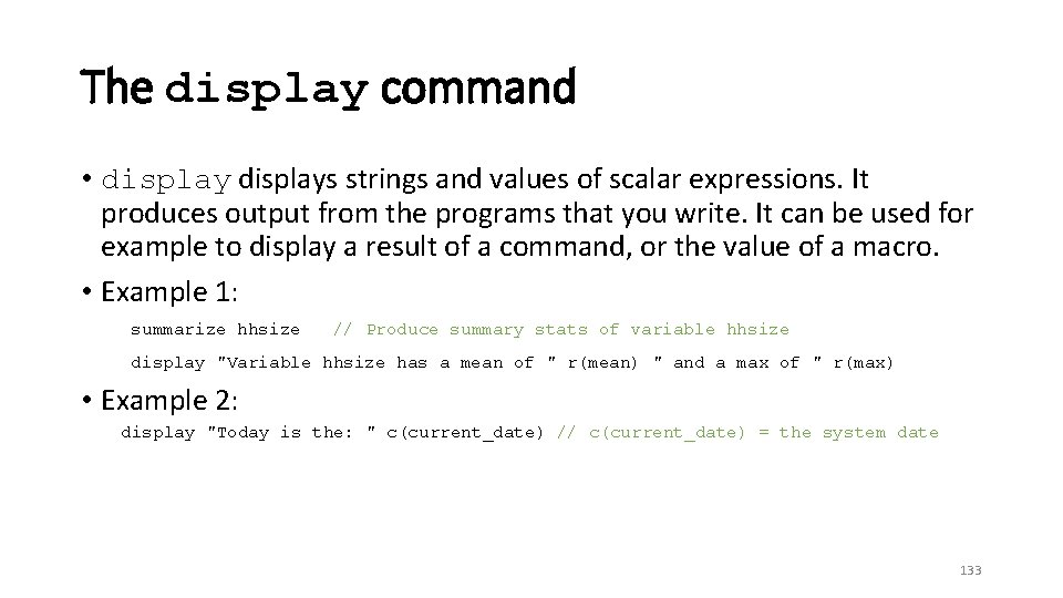
The display command • displays strings and values of scalar expressions. It produces output from the programs that you write. It can be used for example to display a result of a command, or the value of a macro. • Example 1: summarize hhsize // Produce summary stats of variable hhsize display "Variable hhsize has a mean of " r(mean) " and a max of " r(max) • Example 2: display "Today is the: " c(current_date) // c(current_date) = the system date 133

Loops • Many programs will contain commands or sets of commands that need to be repeated (e. g. , you may need to calculate values for each year in a range of years). • Stata provides various methods for looping or repeating commands in a do-file. • Depending on the purpose of the loop, you may want to chose one of the methods over another one (in some cases, more than one method may achieve the same result, but one may be more “elegant” or efficient than another one). 134

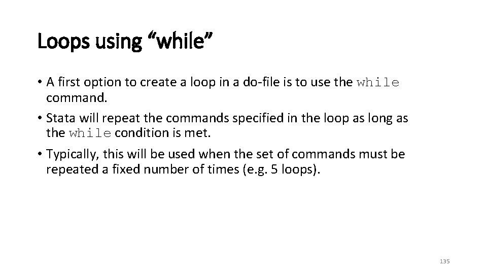
Loops using “while” • A first option to create a loop in a do-file is to use the while command. • Stata will repeat the commands specified in the loop as long as the while condition is met. • Typically, this will be used when the set of commands must be repeated a fixed number of times (e. g. 5 loops). 135

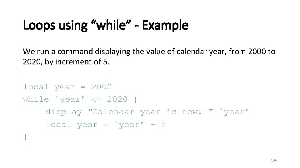
Loops using “while” Example We run a command displaying the value of calendar year, from 2000 to 2020, by increment of 5. local year = 2000 while `year’ <= 2020 { display "Calendar year is now: " `year’ local year = `year’ + 5 } 136

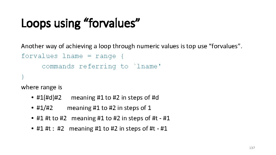
Loops using “forvalues” Another way of achieving a loop through numeric values is top use “forvalues”. forvalues lname = range { commands referring to `lname' } where range is • #1(#d)#2 meaning #1 to #2 in steps of #d • #1/#2 meaning #1 to #2 in steps of 1 • #1 #t to #2 meaning #1 to #2 in steps of #t - #1 • #1 #t : #2 meaning #1 to #2 in steps of #t - #1 137

Loops using “foreach” foreach is used in conjunction with strings. foreach country in KIR FSM FJI { display "The selected country is " "`country'" } This command can be used with variable names, numbers, or any string of text. 138

Loops using “levelsof” • levelsof displays a sorted list of the distinct values of a categorical variable. Using this command, you can generate a macro containing a list of these values, and use this list to loop through the values. • Example: levelsof ethnicgrp, local(ethnic) foreach l of local ethnic { … some commands to be run for each value of ethnic } 139

Branching We may want to execute some commands when a particular condition is met, and another set of commands when the condition is not met. This is done by “branching” using the “if” and “else” commands. The implementation in Stata is as follows: if [condition] { … execute these commands … } else { … execute these other commands … } Notice the use of curly brackets { and }. The set of commands to be implemented under each condition must be listed in their own set of brackets. 140

Preserving and restoring data in memory • preserve and restore deal with the programming problem where the user’s data must be changed to achieve the desired result but, when the program concludes, the programmer wishes to undo the damage done to the data. • When preserve is issued, the user’s data are preserved. The data in memory remain unchanged. When the program or do-file concludes, the user’s data are automatically restored. • After a preserve, the programmer can also instruct Stata to restore the data now with the restore command. This is useful when the programmer needs the original data back and knows that no more damage will be done to the data. • restore, preserve can be used when the programmer needs the data back but plans further damage. restore, not can be used when the programmer wishes to cancel the previous preserve and to have the data currently in memory returned to the user. (Description extracted from the Stata manual) 141

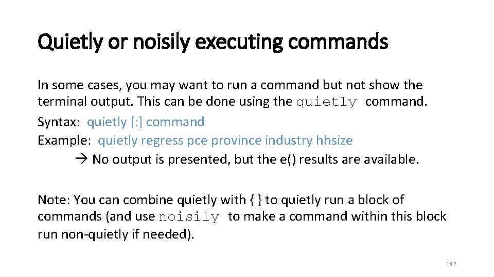
Quietly or noisily executing commands In some cases, you may want to run a command but not show the terminal output. This can be done using the quietly command. Syntax: quietly [: ] command Example: quietly regress pce province industry hhsize No output is presented, but the e() results are available. Note: You can combine quietly with { } to quietly run a block of commands (and use noisily to make a command within this block run non-quietly if needed). 142

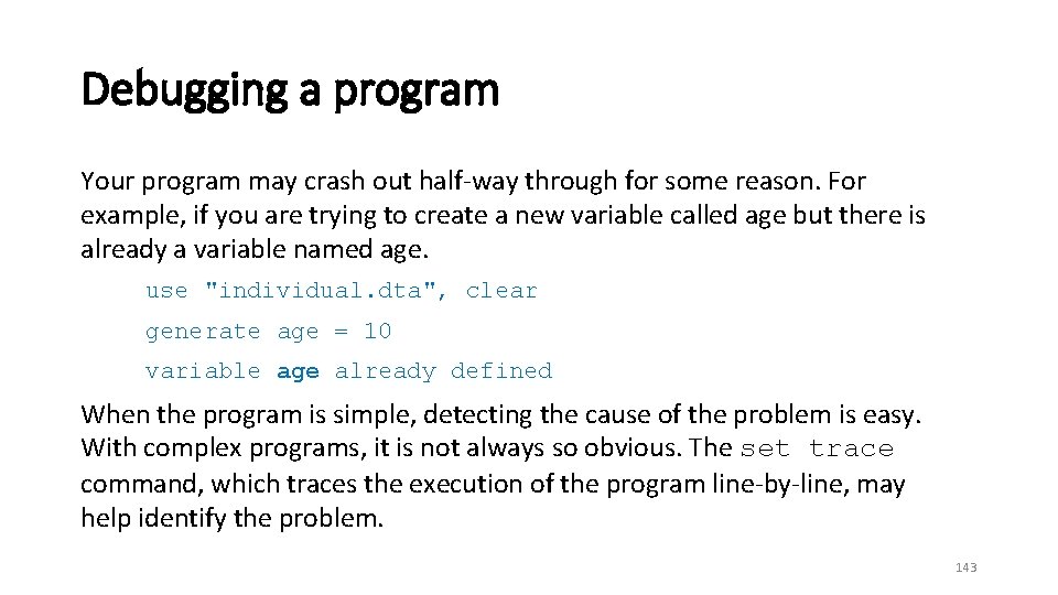
Debugging a program Your program may crash out half-way through for some reason. For example, if you are trying to create a new variable called age but there is already a variable named age. use "individual. dta", clear generate age = 10 variable age already defined When the program is simple, detecting the cause of the problem is easy. With complex programs, it is not always so obvious. The set trace command, which traces the execution of the program line-by-line, may help identify the problem. 143

Working with CSV and Excel files 144

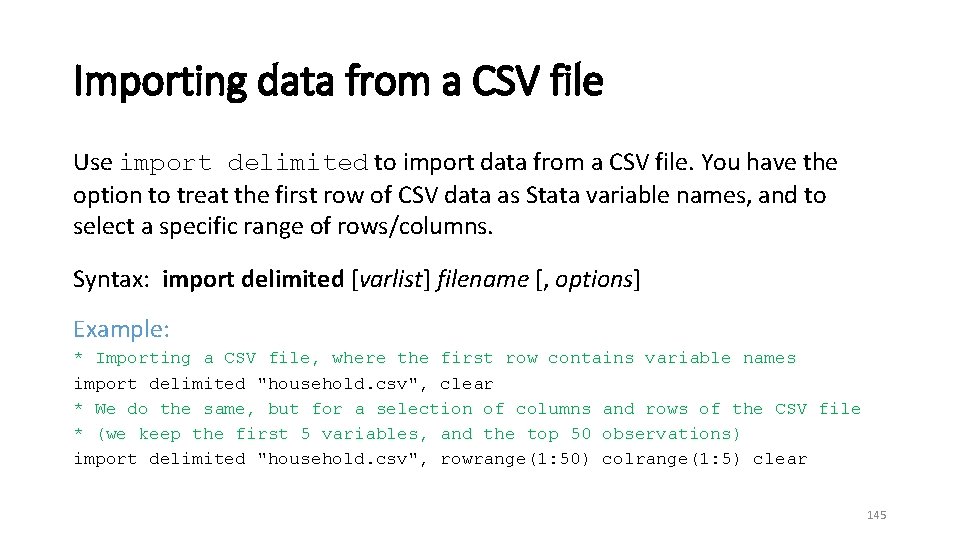
Importing data from a CSV file Use import delimited to import data from a CSV file. You have the option to treat the first row of CSV data as Stata variable names, and to select a specific range of rows/columns. Syntax: import delimited [varlist] filename [, options] Example: * Importing a CSV file, where the first row contains variable names import delimited "household. csv", clear * We do the same, but for a selection of columns and rows of the CSV file * (we keep the first 5 variables, and the top 50 observations) import delimited "household. csv", rowrange(1: 50) colrange(1: 5) clear 145

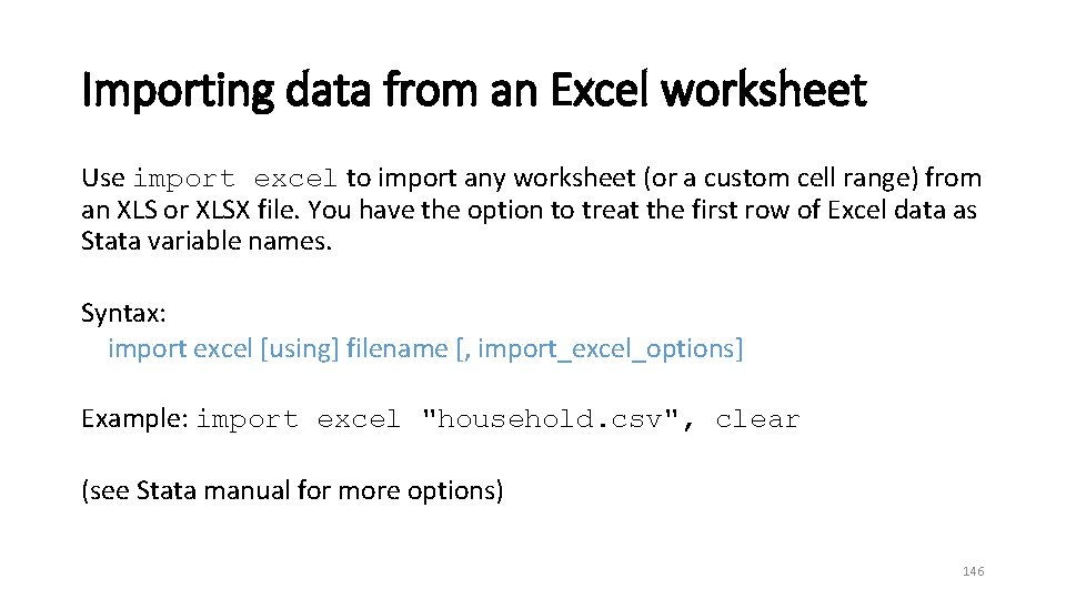
Importing data from an Excel worksheet Use import excel to import any worksheet (or a custom cell range) from an XLS or XLSX file. You have the option to treat the first row of Excel data as Stata variable names. Syntax: import excel [using] filename [, import_excel_options] Example: import excel "household. csv", clear (see Stata manual for more options) 146

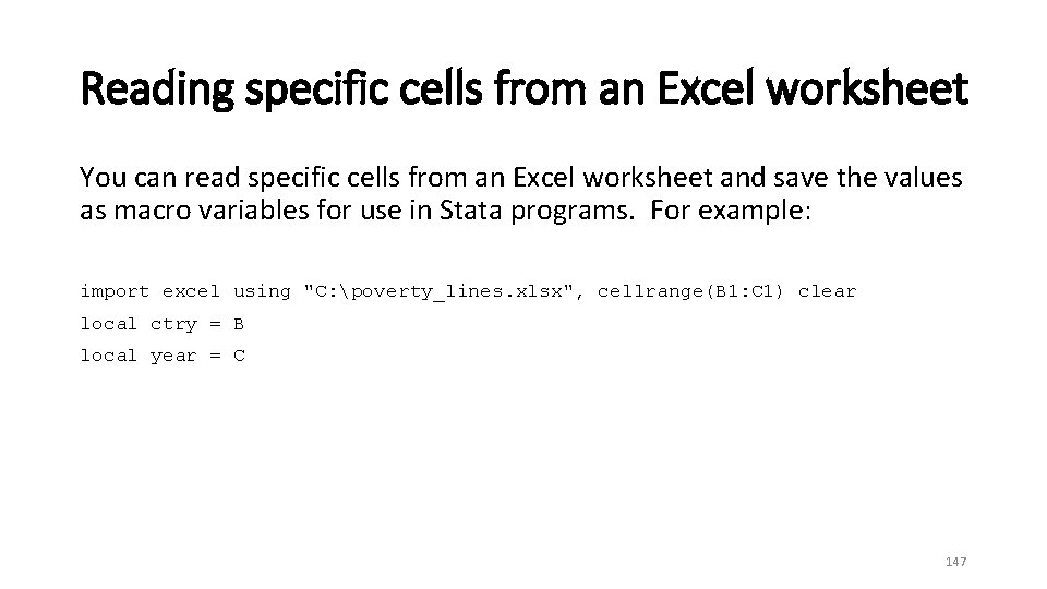
Reading specific cells from an Excel worksheet You can read specific cells from an Excel worksheet and save the values as macro variables for use in Stata programs. For example: import excel using "C: poverty_lines. xlsx", cellrange(B 1: C 1) clear local ctry = B local year = C 147

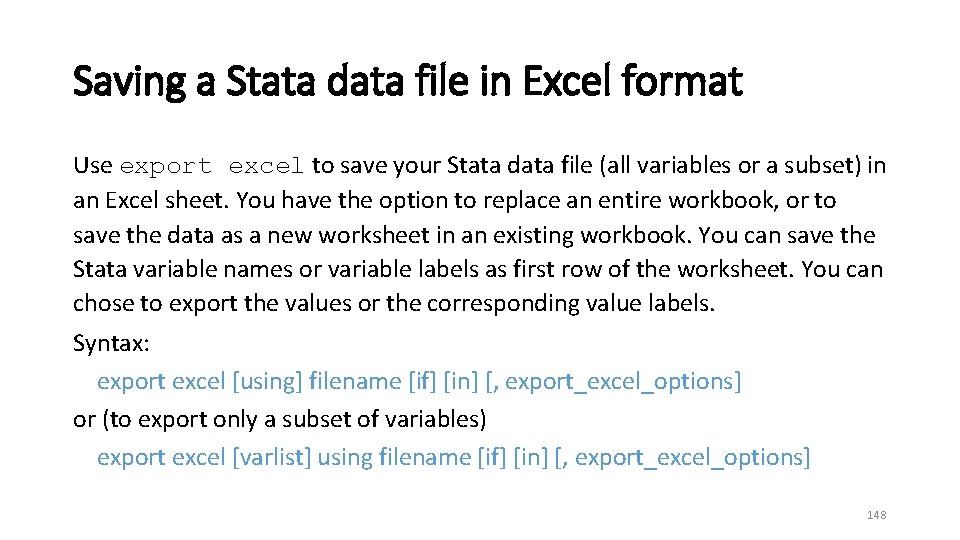
Saving a Stata data file in Excel format Use export excel to save your Stata data file (all variables or a subset) in an Excel sheet. You have the option to replace an entire workbook, or to save the data as a new worksheet in an existing workbook. You can save the Stata variable names or variable labels as first row of the worksheet. You can chose to export the values or the corresponding value labels. Syntax: export excel [using] filename [if] [in] [, export_excel_options] or (to export only a subset of variables) export excel [varlist] using filename [if] [in] [, export_excel_options] 148

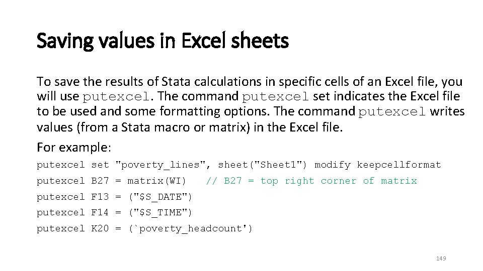
Saving values in Excel sheets To save the results of Stata calculations in specific cells of an Excel file, you will use putexcel. The command putexcel set indicates the Excel file to be used and some formatting options. The command putexcel writes values (from a Stata macro or matrix) in the Excel file. For example: putexcel set "poverty_lines", sheet("Sheet 1") modify keepcellformat putexcel B 27 = matrix(WI) // B 27 = top right corner of matrix putexcel F 13 = ("$S_DATE") putexcel F 14 = ("$S_TIME") putexcel K 20 = (`poverty_headcount') 149

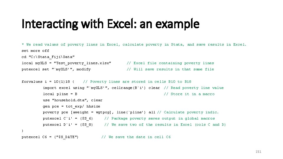
Interacting with Excel: an example In this example, we will extract the value of various poverty lines from an Excel sheet, use these poverty lines to calculate poverty indicators, and save selected poverty indicators back in the XLSX file. Note 1: to run the example shown in the next slide, the package poverty must have been installed (ssc install poverty). Note 2: the package poverty saves the various results it produces in global macros named S_1 to S_27 (see package help file). Global macros are referred to as $S_1 to $S_27 in Stata programs. 150

Interacting with Excel: an example * We read values of poverty lines in Excel, calculate poverty in Stata, and save results in Excel. set more off cd "C: Stata_FijiData" local my. XLS = "Test_poverty_lines. xlsx" // Excel file containing poverty lines putexcel set "`my. XLS'", modify // Will save results in that same file forvalues i = 10(1)18 { // Poverty lines are stored in cells B 10 to B 18 import excel using "`my. XLS'", cellrange(B`i') clear // Read poverty line value local pline = B // Store it in a macro use "household. dta", clear gen pce = tot_exp/ hhsize poverty pce [aweight = wgtpop], line(`pline') all // Calculate poverty indic. putexcel C`i' = ($S_6) // Package poverty saves output in global macros putexcel D`i' = ($S_8) // We save two of the results in Excel (cols C and D) } putexcel C 6 = ("$S_DATE") // We save the date in cell C 6 151

Interacting with the Operating System 152

Interaction with the operating system In some programs, you may want to execute some commands from the operating command prompt, for example to erase a file or to obtain a list of files in a directory. You can execute such commands py preceding them with a ! Examples: !dir C: FSM !erase "C: FSMtemporary_file. dta" 153

Specific commands for survey data tabulation and analysis 154

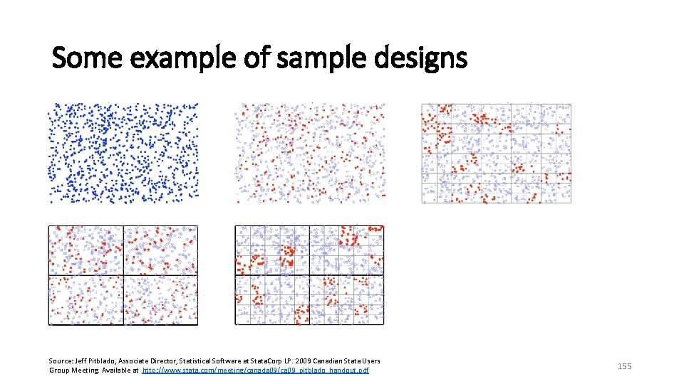
Some example of sample designs Source: Jeff Pitblado, Associate Director, Statistical Software at Stata. Corp LP. 2009 Canadian Stata Users Group Meeting. Available at http: //www. stata. com/meeting/canada 09/ca 09_pitblado_handout. pdf 155

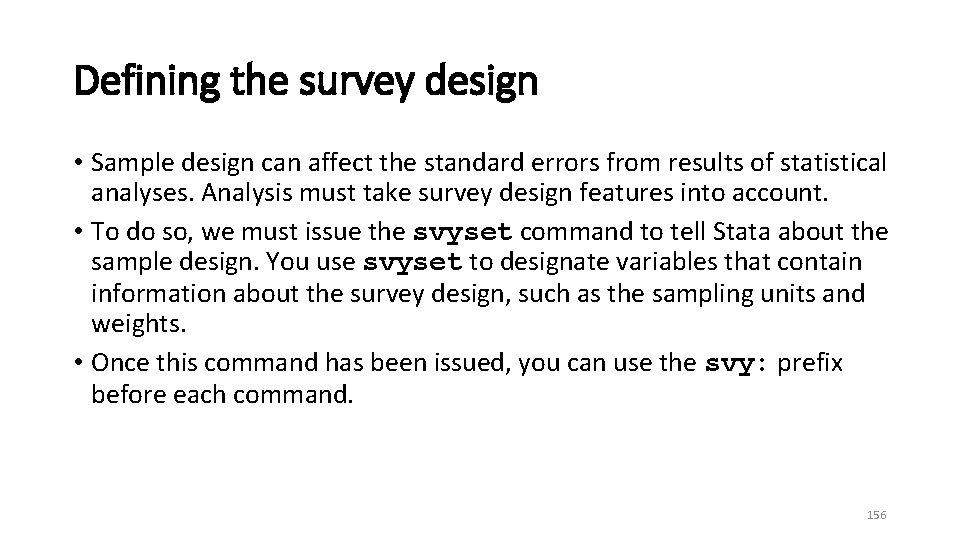
Defining the survey design • Sample design can affect the standard errors from results of statistical analyses. Analysis must take survey design features into account. • To do so, we must issue the svyset command to tell Stata about the sample design. You use svyset to designate variables that contain information about the survey design, such as the sampling units and weights. • Once this command has been issued, you can use the svy: prefix before each command. 156

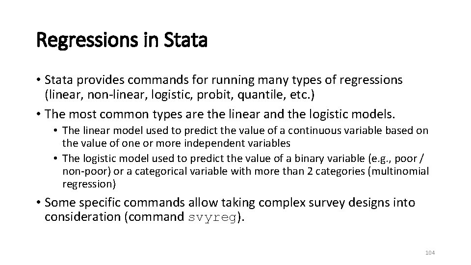
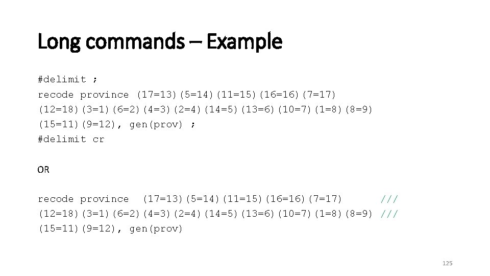
Defining the survey design Syntax • For single-stage design: svyset [psu] [weight] [, design_options] • For multiple-stage design svyset psu [weight] [, design_options] [|| ssu , design_options]. . . [options] 157

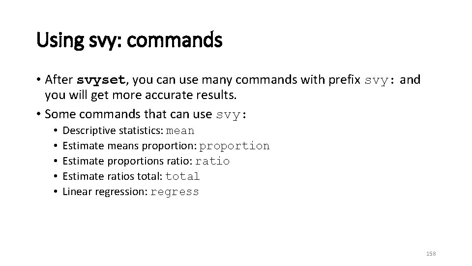
Using svy: commands • After svyset, you can use many commands with prefix svy: and you will get more accurate results. • Some commands that can use svy: • • • Descriptive statistics: mean Estimate means proportion: proportion Estimate proportions ratio: ratio Estimate ratios total: total Linear regression: regress 158

Importing data from Cs. Pro 159

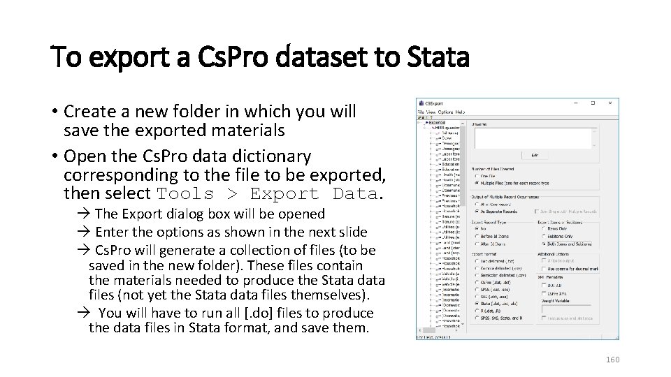
To export a Cs. Pro dataset to Stata • Create a new folder in which you will save the exported materials • Open the Cs. Pro data dictionary corresponding to the file to be exported, then select Tools > Export Data. The Export dialog box will be opened Enter the options as shown in the next slide Cs. Pro will generate a collection of files (to be saved in the new folder). These files contain the materials needed to produce the Stata data files (not yet the Stata data files themselves). You will have to run all [. do] files to produce the data files in Stata format, and save them. 160

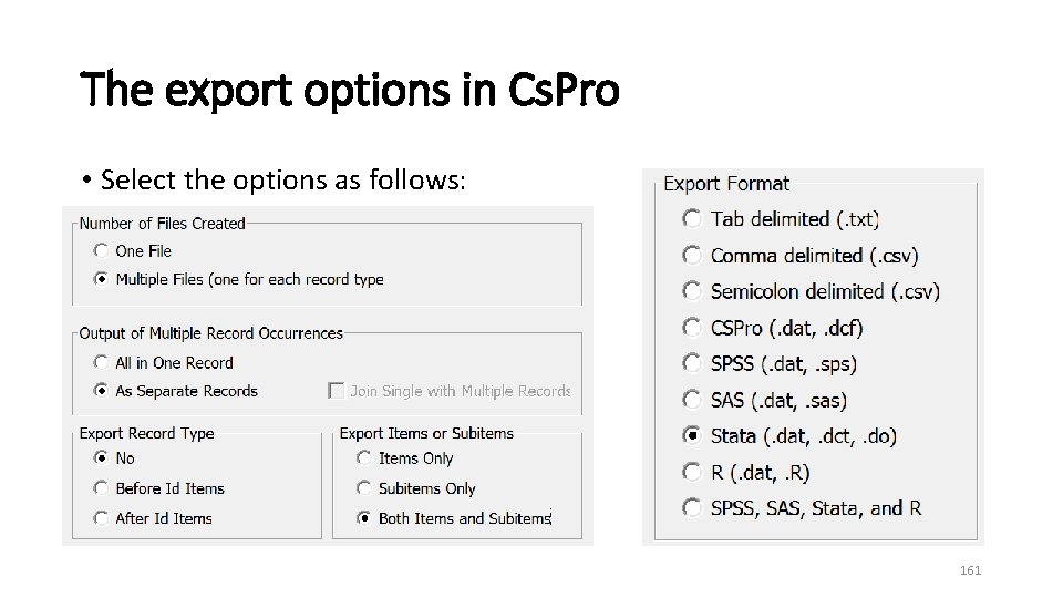
The export options in Cs. Pro • Select the options as follows: 161

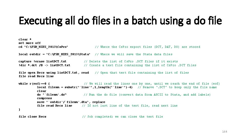
Cs. Pro export to Stata • Cs. Pro export to Stata will generate, for each record type in the Cs. Pro dictionary: • One do file (extension DO) • One dictionary file (extension DCT) • One data file (extension DAT) • Cs. Pro does not generate the Stata data files; it generates the materials needed to produce the Stata data files. • This can involve executing many do files (one per record type). • They can be run one by one, or a do file can be produced to run them in one batch 162

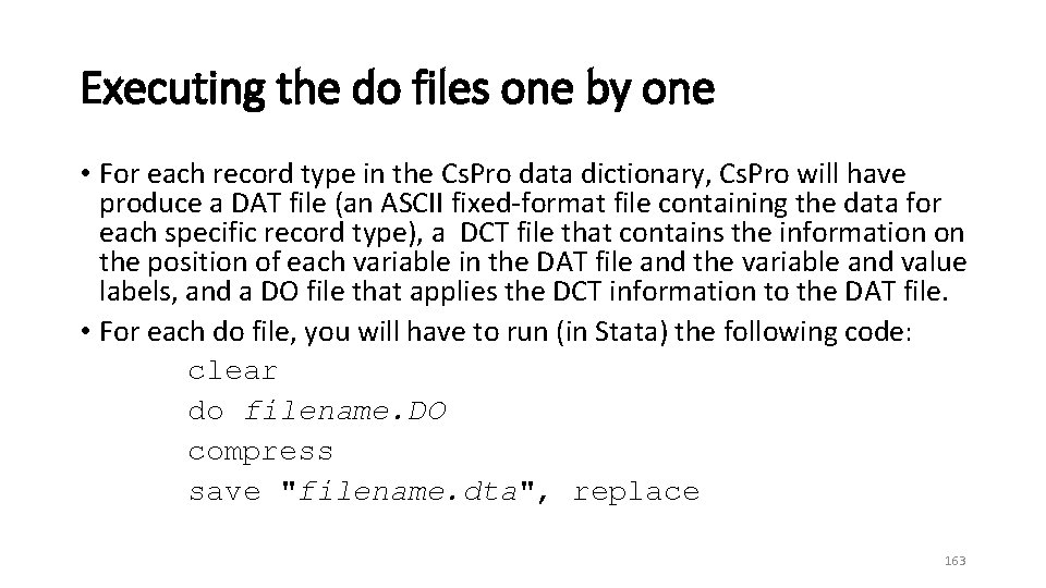
Executing the do files one by one • For each record type in the Cs. Pro data dictionary, Cs. Pro will have produce a DAT file (an ASCII fixed-format file containing the data for each specific record type), a DCT file that contains the information on the position of each variable in the DAT file and the variable and value labels, and a DO file that applies the DCT information to the DAT file. • For each do file, you will have to run (in Stata) the following code: clear do filename. DO compress save "filename. dta", replace 163

Executing all do files in a batch using a do file clear * set more off cd "C: FSM_HIES_2013Cs. Pro" // Where the Cs. Pro export files (DCT, DAT, DO) are stored local outdir = "C: FSM_HIES_2013Stata" // Where we will save the Stata data files capture !erase list. DCT. txt !dir *. dct /B -> list. DCT. txt // Delete the list of Cs. Pro. DCT files if it exists // Create a text file containing the list of Cs. Pro. DCT files file open Recs using list. DCT. txt, read file read Recs line // Open that text file containing the list of files while r(eof)==0 { // We will read the lines one by one, until we reach the end of file (eof) local filenm = substr("`line'", 1, length("`line'")-4) // Remove “. DCT” to keep only the file name clear do "`filenm'. do“ // Run the do file (convert data from ASCII to Stata, and add labels) compress save "`outdir'/`filenm'. dta", replace file read Recs line // If not last line of the text file, read next line } file close Recs // Job completed; we can close the text file 164