An Introduction To Neural Networks Part I Lecture

An Introduction To Neural Networks Part I Lecture 8 Reference(s): An Introduction to Neural Networks for Beginners, Dr. Andy Thomas (Adventures in Machine Learning). Artificial Intelligence: A Guide to Intelligence Systems, Michael Negnevitsky, 3 rd Edition, 2011, Addison Wesley, ISBN 978 -1408225745 Asst. Prof. Dr. Anilkumar K. G 1

Introduction to Neural Networks • An artificial neural network (ANN) or neural network (NN) is a software implementations of the neuronal structure of a human brain. • The brain contains neurons which are kind of like biological switches. – These can change their output state depending on the strength of their electrical or chemical input. – The NN in a person’s brain is a hugely interconnected network of neurons, where the output of any given neuron may be the input to thousands of other neurons (massively parallel structure!). Asst. Prof. Dr. Anilkumar K. G 2

Introduction to Neural Networks • Neural learning occurs by repeatedly activating certain neural connections over others, and this reinforces those connections. • This makes them more likely to produce a desired outcome given a specified input – This learning involves feedback – when the desired outcome occurs, the neural connections causing that outcome becomes strengthened. Asst. Prof. Dr. Anilkumar K. G 3

Introduction to Neural Networks • NNs attempt to simplify and mimic the brain behavior. • They can be trained in a supervised or unsupervised learning manner. • In a supervised NN, the network is trained by providing matched input-output data samples, with the intention of getting the ANN to provide a desired output for a given input. Asst. Prof. Dr. Anilkumar K. G 4

Supervised NN An Example • Consider an e-mail spam filter – the input training data could be the count of various words in the body of the email, and the output training data would be a classification of whether the e-mail was truly spam or not. • If many examples of e-mails are passed through the NN allows the network to learn what input data makes it likely that an e-mail is spam or not. • This learning takes place by adjusting the weights of the NN connections. Asst. Prof. Dr. Anilkumar K. G 5

Unsupervised NN • Unsupervised learning in an NN is an attempt to get the NN to “understand” and generate output structure of the provided input data “on its own”. – There is no supervised learning Asst. Prof. Dr. Anilkumar K. G 6

Structure of an Artificial Neuron • The neurons that we are going to see here are not biological but are Artificial Neurons • The artificial Neurons are extremely simple abstractions of biological neurons, realized as elements in a program or perhaps as a circuit made of silicon. • Networks of these artificial neurons do not have a fraction of the power of the human brain, but they can merely be trained to perform useful functions. Asst. Prof. Dr. Anilkumar K. G 7

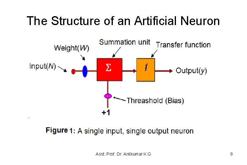
The Structure of an Artificial Neuron • A single-input, single-output artificial neuron is shown in figure 1. • The scalar input N is multiplied by the scalar weight W to form W*N, one of the terms that is sent to the summer unit: – Where N = {n 1, n 2, n 3, …} and W = {w 1, w 2, w 3, …. } – The summer output is often referred to as the net input, and it incorporate with a threshold (or bias), which is the weight of the +1 bias element goes into a transfer function (or activation function) f, which determines and produces the scalar neuron output y. Asst. Prof. Dr. Anilkumar K. G 8

The Structure of an Artificial Neuron Asst. Prof. Dr. Anilkumar K. G 9

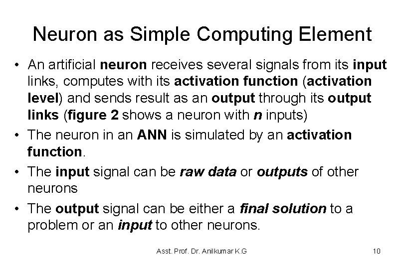
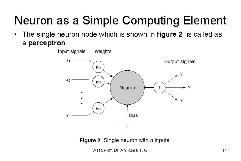
Neuron as Simple Computing Element • An artificial neuron receives several signals from its input links, computes with its activation function (activation level) and sends result as an output through its output links (figure 2 shows a neuron with n inputs) • The neuron in an ANN is simulated by an activation function. • The input signal can be raw data or outputs of other neurons • The output signal can be either a final solution to a problem or an input to other neurons. Asst. Prof. Dr. Anilkumar K. G 10

Neuron as a Simple Computing Element • The single neuron node which is shown in figure 2 is called as a perceptron. Asst. Prof. Dr. Anilkumar K. G 11

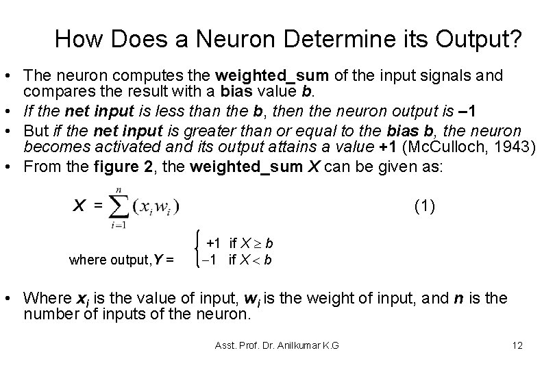
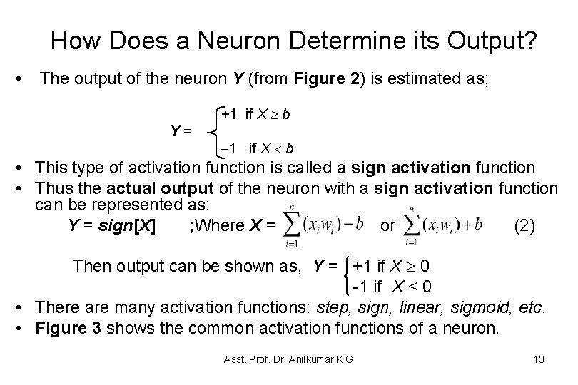
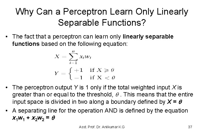
How Does a Neuron Determine its Output? • The neuron computes the weighted_sum of the input signals and compares the result with a bias value b. • If the net input is less than the b, then the neuron output is – 1 • But if the net input is greater than or equal to the bias b, the neuron becomes activated and its output attains a value +1 (Mc. Culloch, 1943) • From the figure 2, the weighted_sum X can be given as: X = where output, Y = (1) +1 if X b • Where xi is the value of input, wi is the weight of input, and n is the number of inputs of the neuron. Asst. Prof. Dr. Anilkumar K. G 12

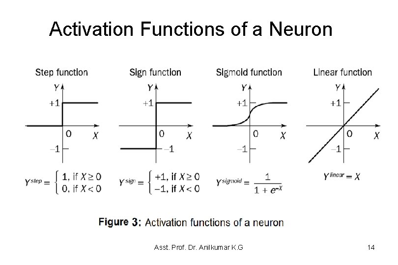
How Does a Neuron Determine its Output? • The output of the neuron Y (from Figure 2) is estimated as; +1 if X b Y= 1 if X b • This type of activation function is called a sign activation function • Thus the actual output of the neuron with a sign activation function can be represented as: Y = sign[X] ; Where X = or (2) Then output can be shown as, Y = +1 if X 0 -1 if X < 0 • There are many activation functions: step, sign, linear, sigmoid, etc. • Figure 3 shows the common activation functions of a neuron. Asst. Prof. Dr. Anilkumar K. G 13

Activation Functions of a Neuron Asst. Prof. Dr. Anilkumar K. G 14

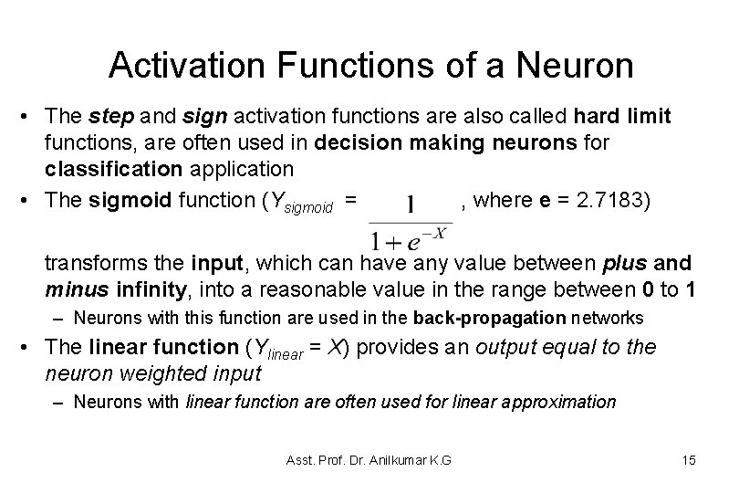
Activation Functions of a Neuron • The step and sign activation functions are also called hard limit functions, are often used in decision making neurons for classification application • The sigmoid function (Ysigmoid = , where e = 2. 7183) transforms the input, which can have any value between plus and minus infinity, into a reasonable value in the range between 0 to 1 – Neurons with this function are used in the back-propagation networks • The linear function (Ylinear = X) provides an output equal to the neuron weighted input – Neurons with linear function are often used for linear approximation Asst. Prof. Dr. Anilkumar K. G 15

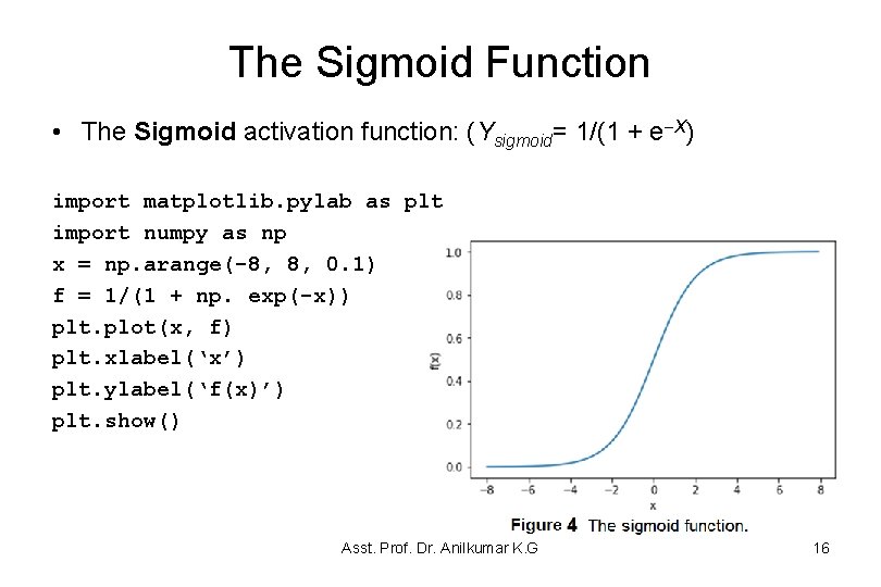
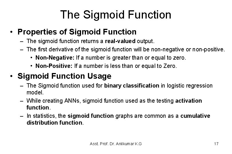
The Sigmoid Function • The Sigmoid activation function: (Ysigmoid= 1/(1 + e X) import matplotlib. pylab as plt import numpy as np x = np. arange(-8, 8, 0. 1) f = 1/(1 + np. exp(-x)) plt. plot(x, f) plt. xlabel(‘x’) plt. ylabel(‘f(x)’) plt. show() Asst. Prof. Dr. Anilkumar K. G 16

The Sigmoid Function • Properties of Sigmoid Function – The sigmoid function returns a real-valued output. – The first derivative of the sigmoid function will be non-negative or non-positive. • Non-Negative: If a number is greater than or equal to zero. • Non-Positive: If a number is less than or equal to Zero. • Sigmoid Function Usage – The Sigmoid function used for binary classification in logistic regression model. – While creating ANNs, sigmoid function used as the testing activation function. – In statistics, the sigmoid function graphs are common as a cumulative distribution function. Asst. Prof. Dr. Anilkumar K. G 17

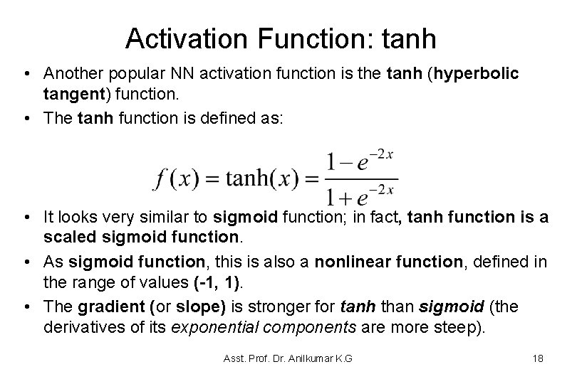
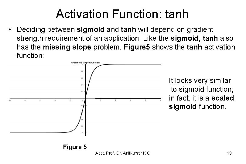
Activation Function: tanh • Another popular NN activation function is the tanh (hyperbolic tangent) function. • The tanh function is defined as: • It looks very similar to sigmoid function; in fact, tanh function is a scaled sigmoid function. • As sigmoid function, this is also a nonlinear function, defined in the range of values (-1, 1). • The gradient (or slope) is stronger for tanh than sigmoid (the derivatives of its exponential components are more steep). Asst. Prof. Dr. Anilkumar K. G 18

Activation Function: tanh • Deciding between sigmoid and tanh will depend on gradient strength requirement of an application. Like the sigmoid, tanh also has the missing slope problem. Figure 5 shows the tanh activation function: It looks very similar to sigmoid function; in fact, it is a scaled sigmoid function. Figure 5 Asst. Prof. Dr. Anilkumar K. G 19

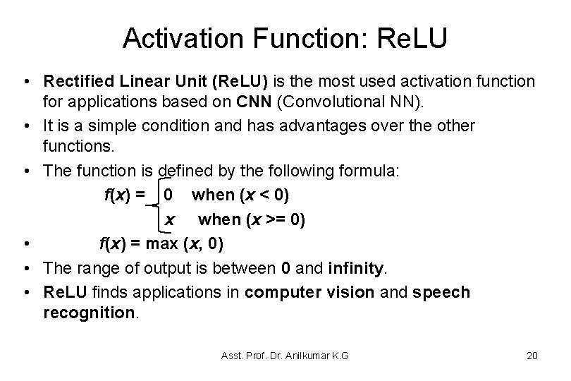
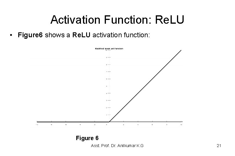
Activation Function: Re. LU • Rectified Linear Unit (Re. LU) is the most used activation function for applications based on CNN (Convolutional NN). • It is a simple condition and has advantages over the other functions. • The function is defined by the following formula: f(x) = 0 when (x < 0) x when (x >= 0) • f(x) = max (x, 0) • The range of output is between 0 and infinity. • Re. LU finds applications in computer vision and speech recognition. Asst. Prof. Dr. Anilkumar K. G 20

Activation Function: Re. LU • Figure 6 shows a Re. LU activation function: Figure 6 Asst. Prof. Dr. Anilkumar K. G 21

Which activation functions to use? • The sigmoid is the most used activation function, but it suffers from the following setbacks: – Since it uses logistic model, the computations are time consuming and complex. – It cause gradients to vanish and no signals pass through the neurons at some point of time. – It is slow in convergence. – It is not zero centered. Asst. Prof. Dr. Anilkumar K. G 22

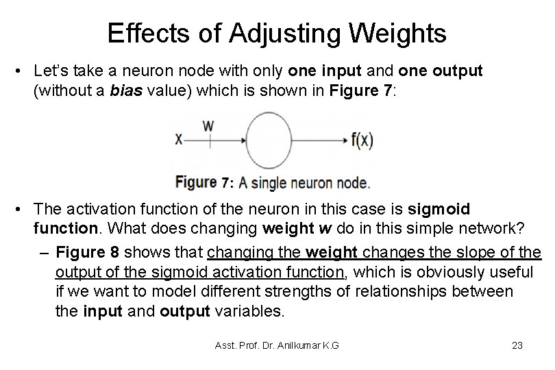
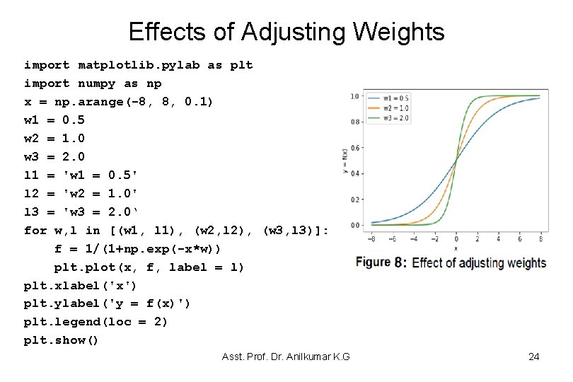
Effects of Adjusting Weights • Let’s take a neuron node with only one input and one output (without a bias value) which is shown in Figure 7: • The activation function of the neuron in this case is sigmoid function. What does changing weight w do in this simple network? – Figure 8 shows that changing the weight changes the slope of the output of the sigmoid activation function, which is obviously useful if we want to model different strengths of relationships between the input and output variables. Asst. Prof. Dr. Anilkumar K. G 23

Effects of Adjusting Weights import matplotlib. pylab as plt import numpy as np x = np. arange(-8, 8, 0. 1) w 1 = 0. 5 w 2 = 1. 0 w 3 = 2. 0 l 1 = 'w 1 = 0. 5' l 2 = 'w 2 = 1. 0' l 3 = 'w 3 = 2. 0‘ for w, l in [(w 1, l 1), (w 2, l 2), (w 3, l 3)]: f = 1/(1+np. exp(-x*w)) plt. plot(x, f, label = l) plt. xlabel('x') plt. ylabel('y = f(x)') plt. legend(loc = 2) plt. show() Asst. Prof. Dr. Anilkumar K. G 24

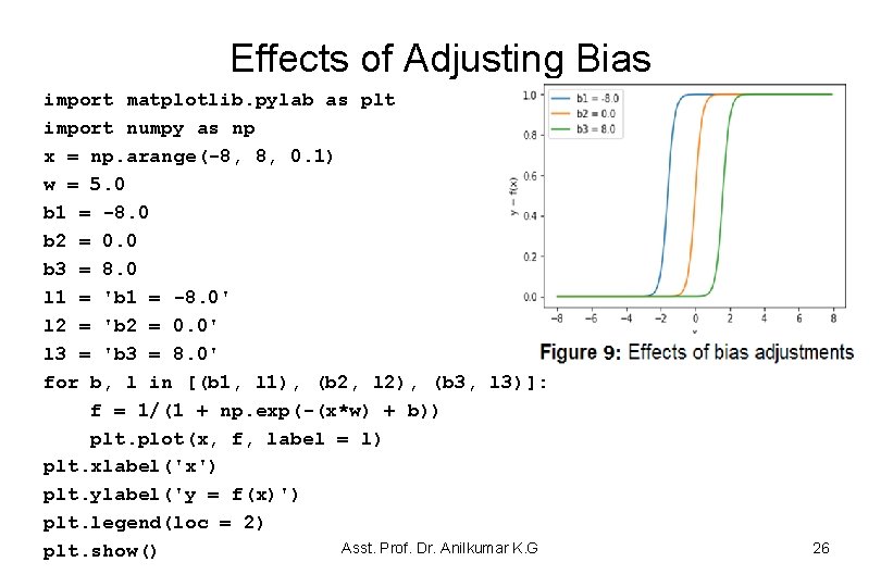
Effects of Adjusting Bias • The weights are real valued numbers, which are multiplied by the inputs and then summed up in the NN node. – In this case, the w has been increased to simulate a more defined “turn on” function. • So, in other words, the weighted input to a neuron node with three inputs (x 1, x 2, and x 3) and their respective weights (w 1, w 2, and w 3) can be: x 1 w 1 + x 2 w 2 + x 3 w 3 + b – where the b is the weight of the +1 bias element of the neuron node, and – the inclusion of this bias weight enhances the flexibility of the neuron node. – The effect of bias adjustment is shown in Figure 9. Asst. Prof. Dr. Anilkumar K. G 25

Effects of Adjusting Bias import matplotlib. pylab as plt import numpy as np x = np. arange(-8, 8, 0. 1) w = 5. 0 b 1 = -8. 0 b 2 = 0. 0 b 3 = 8. 0 l 1 = 'b 1 = -8. 0' l 2 = 'b 2 = 0. 0' l 3 = 'b 3 = 8. 0' for b, l in [(b 1, l 1), (b 2, l 2), (b 3, l 3)]: f = 1/(1 + np. exp(-(x*w) + b)) plt. plot(x, f, label = l) plt. xlabel('x') plt. ylabel('y = f(x)') plt. legend(loc = 2) Asst. Prof. Dr. Anilkumar K. G plt. show() 26

Effects of Adjusting Bias • Figure 9 shows that by varying the bias weight b, you can change the output when the neuron node activates. • Therefore, by adding a bias term, you can make a neuron node simulates a generic if function; – i. e. if (x > z) then 1 else 0. – Without a bias term, you are unable to vary the z of the if statement, it will be always stuck around 0. • This is obviously very useful if you are trying to simulate conditional relationships. Asst. Prof. Dr. Anilkumar K. G 27

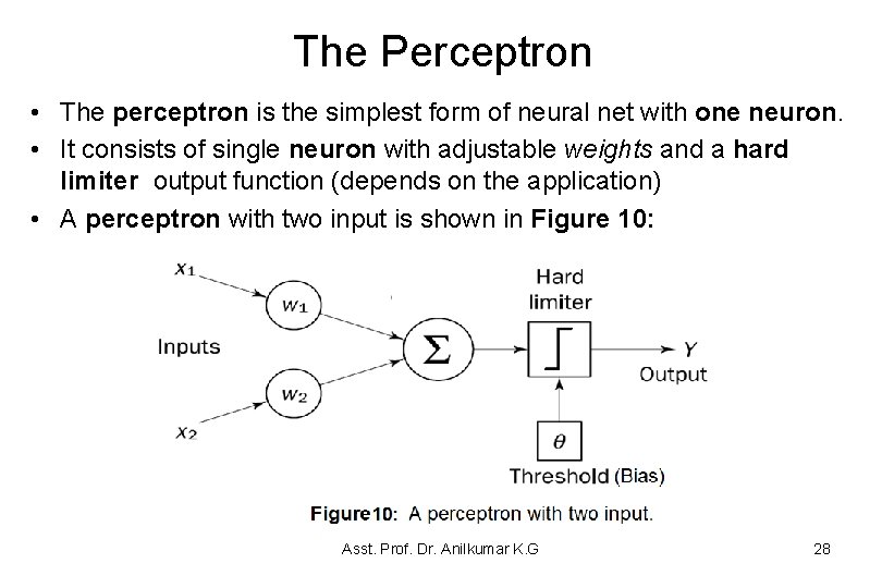
The Perceptron • The perceptron is the simplest form of neural net with one neuron. • It consists of single neuron with adjustable weights and a hard limiter output function (depends on the application) • A perceptron with two input is shown in Figure 10: Asst. Prof. Dr. Anilkumar K. G 28

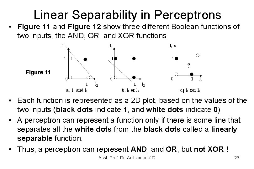
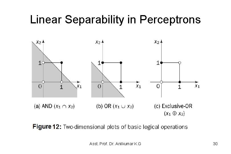
Linear Separability in Perceptrons • Figure 11 and Figure 12 show three different Boolean functions of two inputs, the AND, OR, and XOR functions Figure 11 • Each function is represented as a 2 D plot, based on the values of the two inputs (black dots indicate 1, and white dots indicate 0) • A perceptron can represent a function only if there is some line that separates all the white dots from the black dots called a linearly separable function. • Thus, a perceptron can represent AND, and OR, but not XOR ! Asst. Prof. Dr. Anilkumar K. G 29

Linear Separability in Perceptrons Asst. Prof. Dr. Anilkumar K. G 30

The Perceptron Learning Rule • The perceptron learning rule was first proposed by Rosenblatt in 1960 • Using this rule we can derive the perceptron training algorithm for classification tasks • This is done by making small adjustments in the weights to reduce the difference between the actual (calculated/predicted) and desired (given/expected) outputs of the perceptron. – The initial weights are randomly assigned in the range [-0. 5, 0. 5] and then updated to obtain the output consistent with the training examples Asst. Prof. Dr. Anilkumar K. G 31

The Perceptron Learning Rule • If at iteration p, the calculated/predicted output is Y(p) and the desired output is Yd(p), then the error e at iteration p is given by e(p) = Yd(p) – Y(p), where p = 1, 2, 3, … (3) • If the error e(p) is positive, we need to increase Y(p) • If the error is negative, we need to decrease Y(p) • Taking into the account that each perceptron input contributes xi(p) wi(p) with a base (threashold) to the total input X(p) • Based on this concept, the perceptron learning rule is established: wi(p+1) = wi(p) + xi(p) e(p) (4) Where is the learning rate, a positive constant less than unity Asst. Prof. Dr. Anilkumar K. G 32

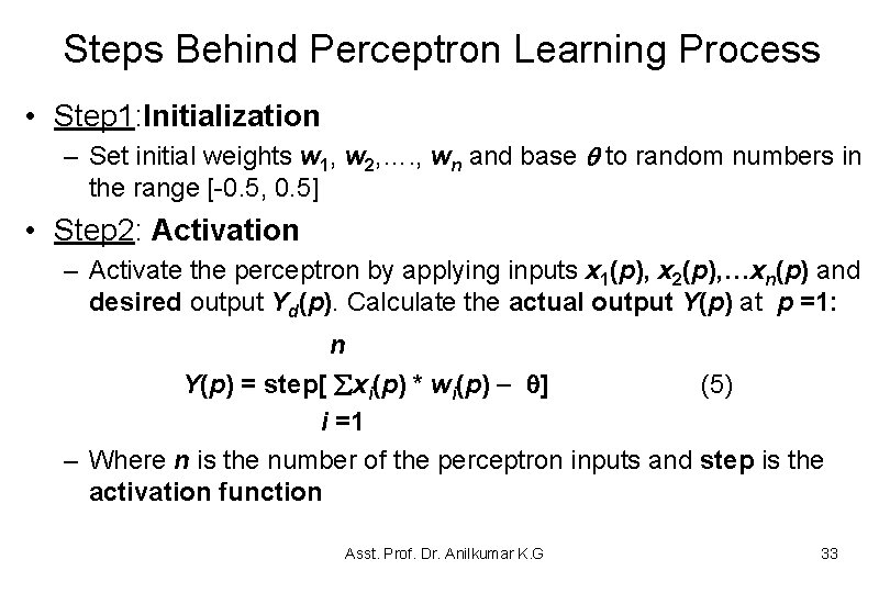
Steps Behind Perceptron Learning Process • Step 1: Initialization – Set initial weights w 1, w 2, …. , wn and base to random numbers in the range [-0. 5, 0. 5] • Step 2: Activation – Activate the perceptron by applying inputs x 1(p), x 2(p), …xn(p) and desired output Yd(p). Calculate the actual output Y(p) at p =1: n Y(p) = step[ xi(p) * wi(p) ] (5) i =1 – Where n is the number of the perceptron inputs and step is the activation function Asst. Prof. Dr. Anilkumar K. G 33

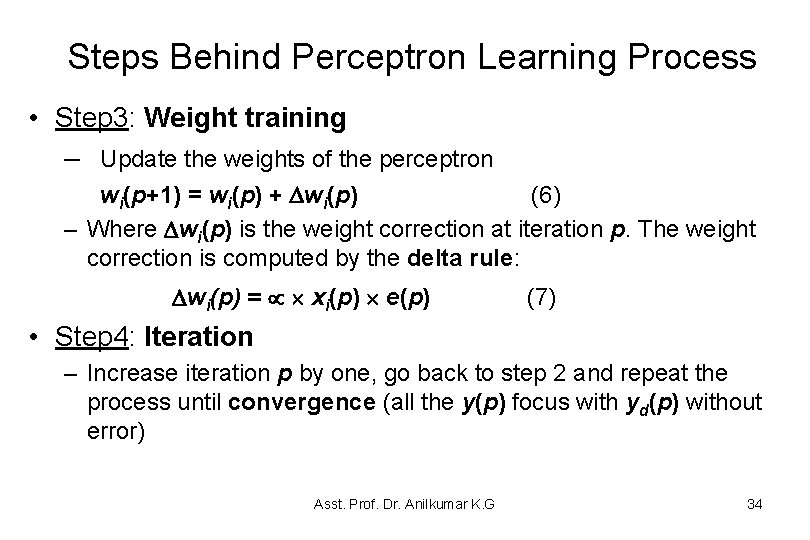
Steps Behind Perceptron Learning Process • Step 3: Weight training – Update the weights of the perceptron wi(p+1) = wi(p) + wi(p) (6) – Where wi(p) is the weight correction at iteration p. The weight correction is computed by the delta rule: wi(p) = xi(p) e(p) (7) • Step 4: Iteration – Increase iteration p by one, go back to step 2 and repeat the process until convergence (all the y(p) focus with yd(p) without error) Asst. Prof. Dr. Anilkumar K. G 34

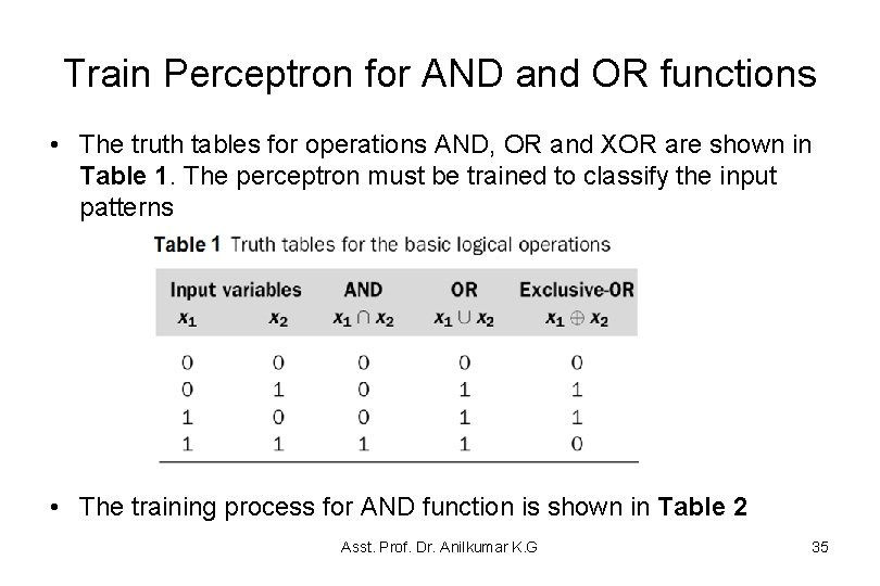
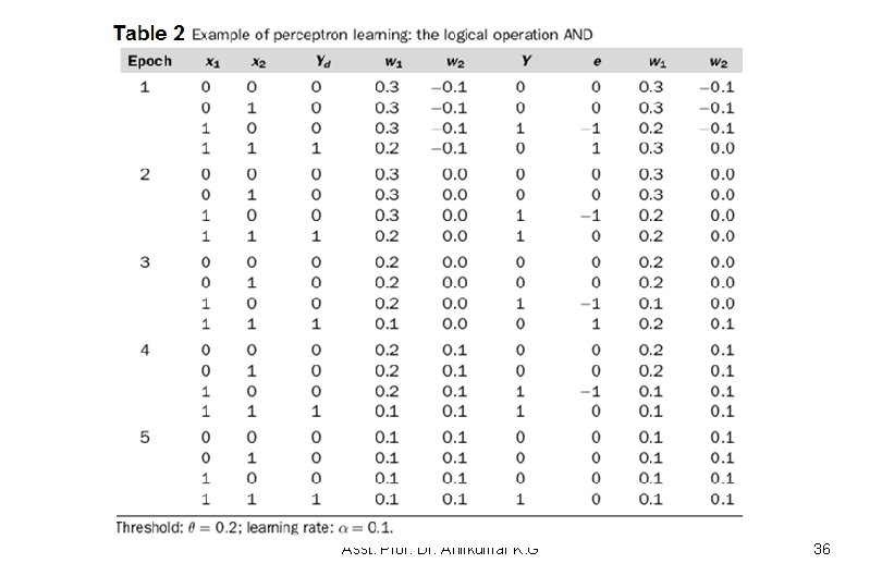
Train Perceptron for AND and OR functions • The truth tables for operations AND, OR and XOR are shown in Table 1. The perceptron must be trained to classify the input patterns • The training process for AND function is shown in Table 2 Asst. Prof. Dr. Anilkumar K. G 35

Asst. Prof. Dr. Anilkumar K. G 36

Why Can a Perceptron Learn Only Linearly Separable Functions? • The fact that a perceptron can learn only linearly separable functions based on the following equation: • The perceptron output Y is 1 only if the total weighted input X is greater than or equal to the threshold, . This means that the entire input space is divided in two along a boundary defined by X = • A separating line for the operation AND is defined by the equation x 1 w 1 + x 2 w 2 = Asst. Prof. Dr. Anilkumar K. G 37

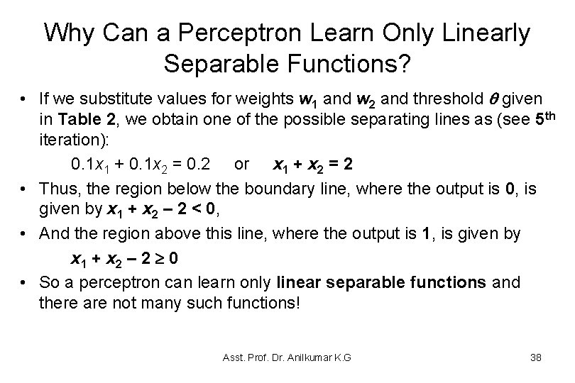
Why Can a Perceptron Learn Only Linearly Separable Functions? • If we substitute values for weights w 1 and w 2 and threshold given in Table 2, we obtain one of the possible separating lines as (see 5 th iteration): 0. 1 x 1 + 0. 1 x 2 = 0. 2 or x 1 + x 2 = 2 • Thus, the region below the boundary line, where the output is 0, is given by x 1 + x 2 – 2 < 0, • And the region above this line, where the output is 1, is given by x 1 + x 2 – 2 0 • So a perceptron can learn only linear separable functions and there are not many such functions! Asst. Prof. Dr. Anilkumar K. G 38

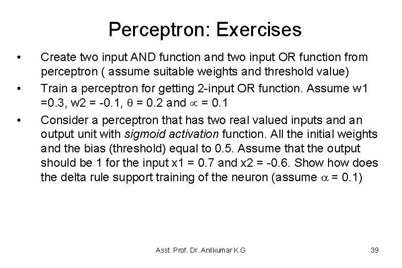
Perceptron: Exercises • • • Create two input AND function and two input OR function from perceptron ( assume suitable weights and threshold value) Train a perceptron for getting 2 -input OR function. Assume w 1 =0. 3, w 2 = -0. 1, = 0. 2 and = 0. 1 Consider a perceptron that has two real valued inputs and an output unit with sigmoid activation function. All the initial weights and the bias (threshold) equal to 0. 5. Assume that the output should be 1 for the input x 1 = 0. 7 and x 2 = -0. 6. Show does the delta rule support training of the neuron (assume = 0. 1) Asst. Prof. Dr. Anilkumar K. G 39

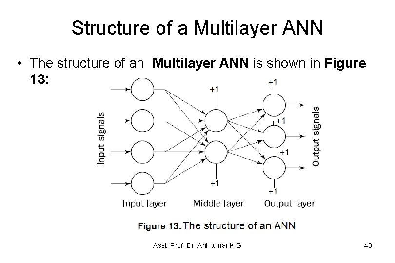
Structure of a Multilayer ANN • The structure of an Multilayer ANN is shown in Figure 13: Asst. Prof. Dr. Anilkumar K. G 40