An Introduction to MODFLOW What is MODFLOW Widely

An Introduction to MODFLOW

What is MODFLOW? § § § Widely used ground-water flow simulation program that runs on any platform (Windows, Sun, Unix, Linux, …). Mostly written in standard FORTRAN (GMG is C++) Solves the ground-water flow equation with different possible properties, boundary conditions, and initial conditions First version, 1983, Mc. Donald and Harbaugh. Written to serve USGS needs. Education emphasized. MODFLOW escaped! Public domain (Free) Open source (Anyone can check and change the source code) Changed versions are sometimes commercial – it’s up to the developer Well documented Modularly constructed (More later) Latest version: MODFLOW-2005 (Harbaugh, 2005)

What is MODFLOW? § Cited in statutes, legally tested § 250, 000 hits on Google for MODFLOW § Many other programs use results from or are based on MODFLOW: § Public domain/open source § MT 3 DMS (multi-species solute or heat transport, some reactions, § § § dual porosity) (Chunmiao Zheng, U Alabama) MODPATH (particle tracking) (Dave Pollock, USGS) SEAWAT (density-dependent transport using MODFLOW and MT 3 DMS) (Chris Langevin, USGS) Phreeqc connections (PHT 3 D) (Henning Prommer) § Commercial § MODHMS-Surfact (Integrated sw/gw/unsat) § GUI’s: Visual MODFLOW, Groundwater Vistas, GMS, PMWin, …

What is MODFLOW? § Program organized into MODules § Activate the capabilities you need; no overhead from other capabilities (execution time, RAM) § The structure is clear and documented for adding additional capabilities such as new equations § Modularity in ‘Processes’ and ‘Packages’ What is MODFLOW-2005? § § § Latest release of USGS MODFLOW Internal computer storage redesigned to support storage of multiple models necessary for local grid refinement and facilitate linkages to other models (GSFLOW = MODFLOW + PRMS). Parameter-estimation, sensitivity analysis, uncertainty now from UCODE_2005

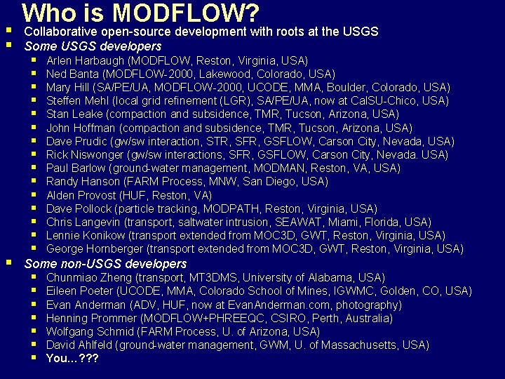
§ § § Who is MODFLOW? Collaborative open-source development with roots at the USGS Some USGS developers § § § § Arlen Harbaugh (MODFLOW, Reston, Virginia, USA) Ned Banta (MODFLOW-2000, Lakewood, Colorado, USA) Mary Hill (SA/PE/UA, MODFLOW-2000, UCODE, MMA, Boulder, Colorado, USA) Steffen Mehl (local grid refinement (LGR), SA/PE/UA, now at Cal. SU-Chico, USA) Stan Leake (compaction and subsidence, TMR, Tucson, Arizona, USA) John Hoffman (compaction and subsidence, TMR, Tucson, Arizona, USA) Dave Prudic (gw/sw interaction, STR, SFR, GSFLOW, Carson City, Nevada, USA) Rick Niswonger (gw/sw interactions, SFR, GSFLOW, Carson City, Nevada. USA) Paul Barlow (ground-water management, MODMAN, Reston, VA, USA) Randy Hanson (FARM Process, MNW, San Diego, USA) Alden Provost (HUF, Reston, VA) Dave Pollock (particle tracking, MODPATH, Reston, Virginia, USA) Chris Langevin (transport, saltwater intrusion, SEAWAT, Miami, Florida, USA) Lennie Konikow (transport extended from MOC 3 D, GWT, Reston, Virginia, USA) George Hornberger (transport extended from MOC 3 D, GWT, Reston, Virginia, USA) Some non-USGS developers § § § § Chunmiao Zheng (transport, MT 3 DMS, University of Alabama, USA) Eileen Poeter (UCODE, MMA, Colorado School of Mines, IGWMC, Golden, CO, USA) Evan Anderman (ADV, HUF, now at Evan. Anderman. com, photography) Henning Prommer (MODFLOW+PHREEQC, CSIRO, Perth, Australia) Wolfgang Schmid (FARM Process, U. of Arizona, USA) David Ahlfeld (ground-water management, GWM, U. of Massachusetts, USA) You…? ? ?

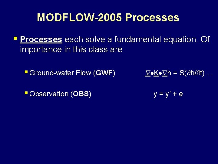
MODFLOW-2005 Processes § Processes each solve a fundamental equation. Of importance in this class are § Ground-water Flow (GWF) § Observation (OBS) K h = S( h/ t) … y = y′ + e

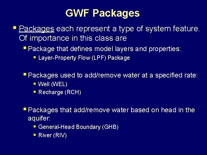
GWF Packages § Packages each represent a type of system feature. Of importance in this class are § Package that defines model layers and properties: § Layer-Property Flow (LPF) Package § Packages used to add/remove water at a specified rate: § Well (WEL) § Recharge (RCH) § Packages that add/remove water based on head in the aquifer: § General-Head Boundary (GHB) § River (RIV)

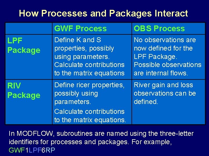
How Processes and Packages Interact GWF Process OBS Process LPF Package Define K and S properties, possibly using parameters. Calculate contributions to the matrix equations No observations are now defined for the LPF Package. Possible observations are internal flows. RIV Package Define ricer properties, possibly using parameters. Calculate contributions to the matrix equations. River gain and loss observations can be defined. In MODFLOW, subroutines are named using the three-letter identifiers for processes and packages. For example, GWF 1 LPF 6 RP

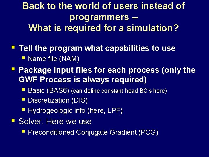
Back to the world of users instead of programmers -What is required for a simulation? § Tell the program what capabilities to use § Name file (NAM) § Package input files for each process (only the GWF Process is always required) § Basic (BAS 6) (can define constant head BC’s here) § Discretization (DIS) § Hydrogeologic info (here, LPF) § Solver. Here we use § Preconditioned Conjugate Gradient (PCG)

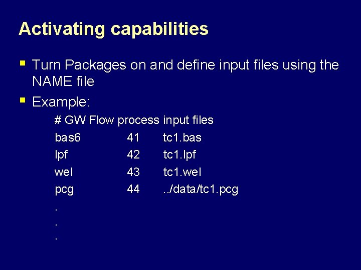
Activating capabilities § § Turn Packages on and define input files using the NAME file Example: # GW Flow process input files bas 6 41 tc 1. bas lpf 42 tc 1. lpf wel 43 tc 1. wel pcg 44. . /data/tc 1. pcg. . .

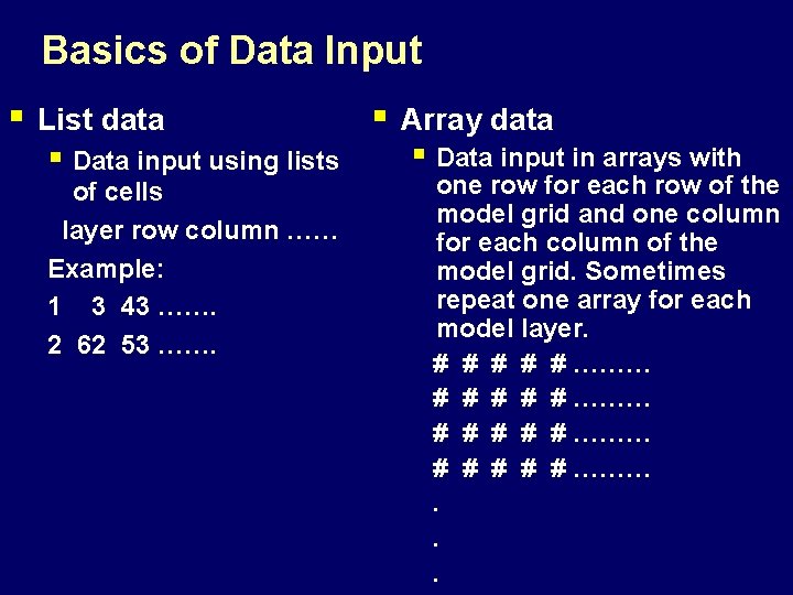
Basics of Data Input § List data § Data input using lists of cells layer row column …… Example: 1 3 43 ……. 2 62 53 ……. § Array data § Data input in arrays with one row for each row of the model grid and one column for each column of the model grid. Sometimes repeat one array for each model layer. # # # # # ………. . .

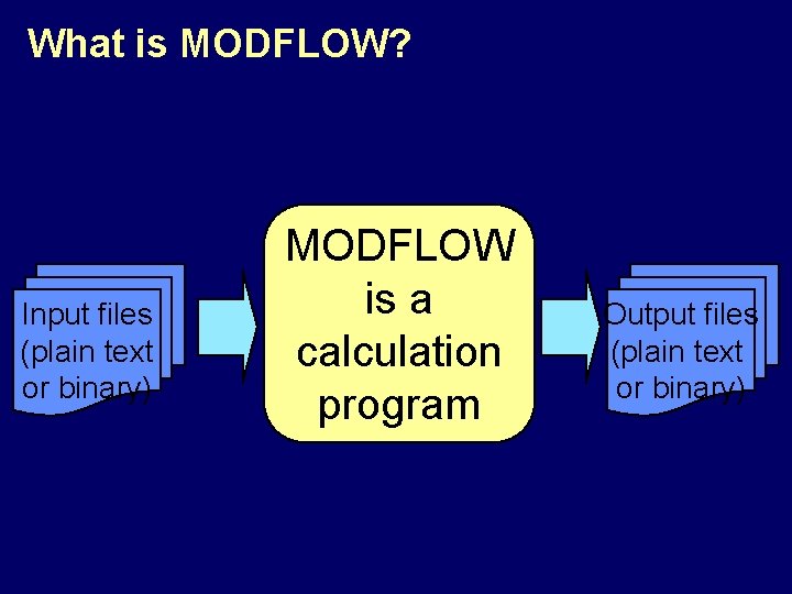
What is MODFLOW? Input files (plain text or binary) MODFLOW is a calculation program Output files (plain text or binary)

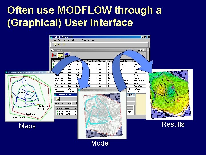
Often use MODFLOW through a (Graphical) User Interface Results Maps Model

§ MODFLOW capabilities used in class Class exercise § MODFLOW Packages used § Layer-Property Flow (LPF) § Recharge (RCH) § River (RIV) § General-Head Boundary (GHB) § Advective Transport (ADV) § Preconditioned-Conjugate Gradient § § (PCG) MODFLOW Processes used § Ground-Water Flow (GWF) § Observations (OBS) UCODE_2005 capabilities used § Sensitivity § Parameter-Estimation

Aspects of flow model creation § Conceptual model § Base map § Grid design § § § § Areal Model layers (thickness can be variable) Boundary conditions Aquifer properties Pumping wells Recharge Time Here, describe selected aspects of capabilities used in class

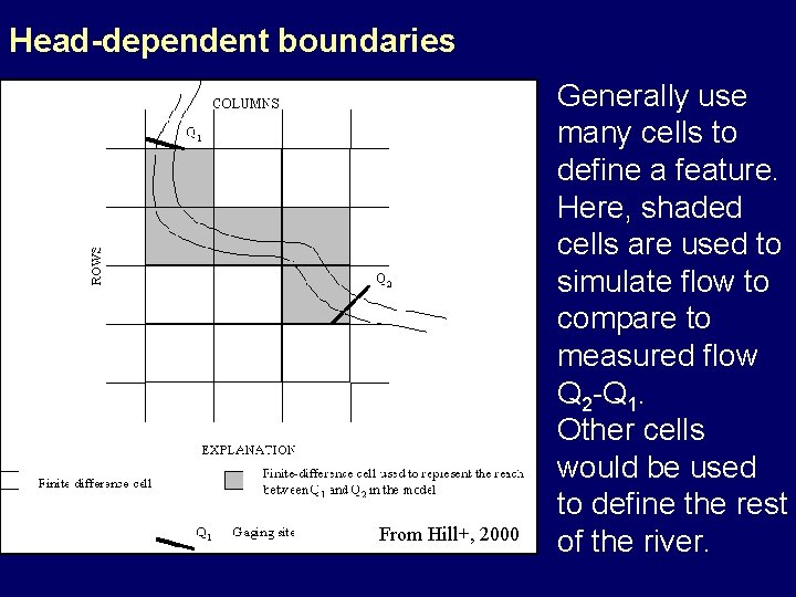
Head-dependent boundaries From Hill+, 2000 Generally use many cells to define a feature. Here, shaded cells are used to simulate flow to compare to measured flow Q 2 -Q 1. Other cells would be used to define the rest of the river.

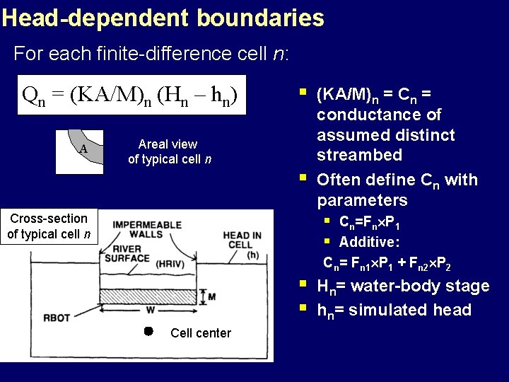
Head-dependent boundaries For each finite-difference cell n: Qn = (KA/M)n (Hn – hn) A Areal view of typical cell n § § (KA/M)n = Cn = conductance of assumed distinct streambed Often define Cn with parameters § § Cross-section of typical cell n § § Cell center Cn=Fn P 1 Additive: Cn= Fn 1 P 1 + Fn 2 P 2 Hn= water-body stage hn= simulated head

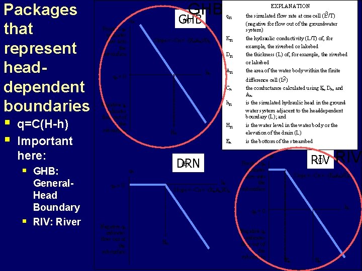
Packages that represent headdependent boundaries § q=C(H-h) § Important GHB (A) GHB qn Positive qn indicates flow into the subsurface Slope = -Cn = -(Kn. An)/Dn § GHB: General. Head Boundary RIV: River qn Kn Dn hn qn = 0 An Cn hn Negative qn indicates flow out of the subsurface Hn Hn En here: § EXPLANATION (B) DRN qn hn Slope = -Cn = -(Kn. An)/Dn qn = 0 the simulated flow rate at one cell (L 3/T) (negative for flow out of the ground-water system) the hydraulic conductivity (L/T) of, for example, the riverbed or lakebed the thickness (L) of, for example, the riverbed or lakebed the area of the water body within the finitedifference cell (L 2) the conductance calculated using Kn, Dn, and An. is the simulated hydraulic head in the groundwater system adjacent to the head-dependent boundary (L); and is the water level in the water body or the (C) elevation of the drain (L) is the bottom of the streambed (C) RIV qn Positive qn indicates flow into the subsurface Slope = -Cn = -(Kn. An)/Dn hn qn = 0 Negative qn indicates flow out of the subsurface Hn Negative qn indicates flow out of the subsurface RIV En Hn

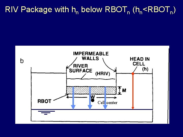
RIV Package with hn below RBOTn (hn<RBOTn) Cell center

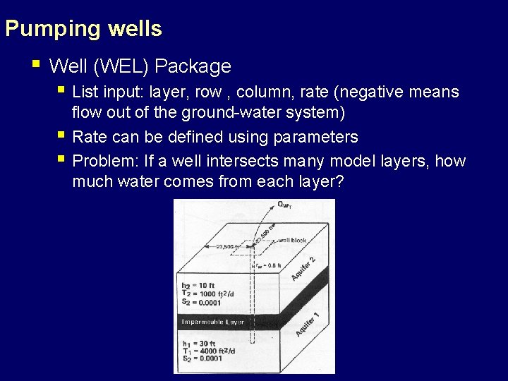
Pumping wells § Well (WEL) Package § List input: layer, row , column, rate (negative means § § flow out of the ground-water system) Rate can be defined using parameters Problem: If a well intersects many model layers, how much water comes from each layer?

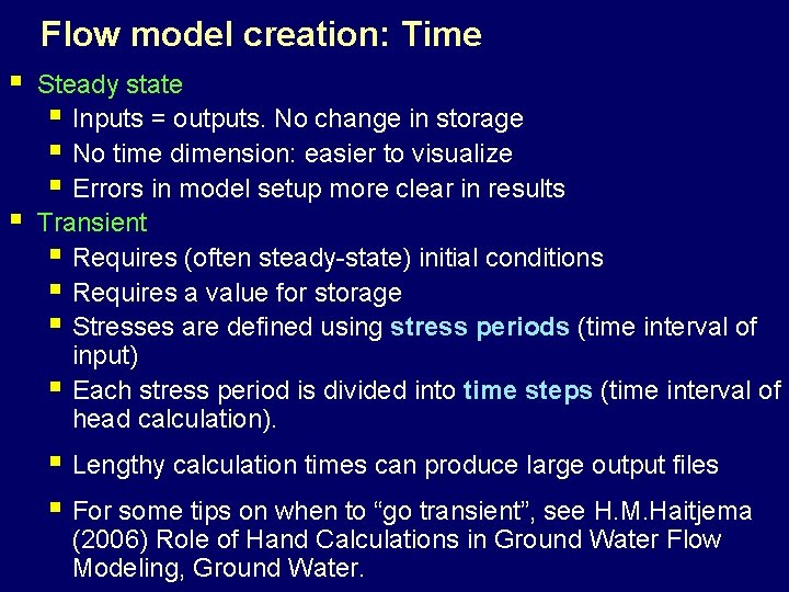
Flow model creation: Time § § Steady state § Inputs = outputs. No change in storage § No time dimension: easier to visualize § Errors in model setup more clear in results Transient § Requires (often steady-state) initial conditions § Requires a value for storage § Stresses are defined using stress periods (time interval of input) § Each stress period is divided into time steps (time interval of head calculation). § Lengthy calculation times can produce large output files § For some tips on when to “go transient”, see H. M. Haitjema (2006) Role of Hand Calculations in Ground Water Flow Modeling, Ground Water.

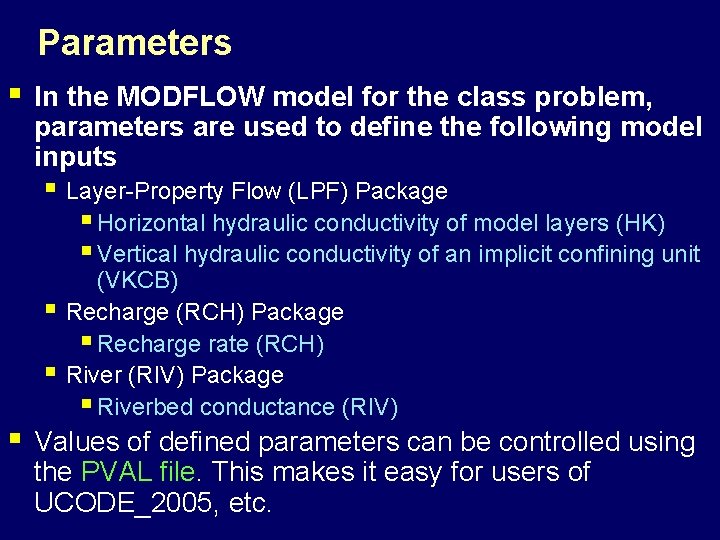
Parameters § In the MODFLOW model for the class problem, parameters are used to define the following model inputs § Layer-Property Flow (LPF) Package § Horizontal hydraulic conductivity of model layers (HK) § Vertical hydraulic conductivity of an implicit confining unit § § § (VKCB) Recharge (RCH) Package § Recharge rate (RCH) River (RIV) Package § Riverbed conductance (RIV) Values of defined parameters can be controlled using the PVAL file. This makes it easy for users of UCODE_2005, etc.

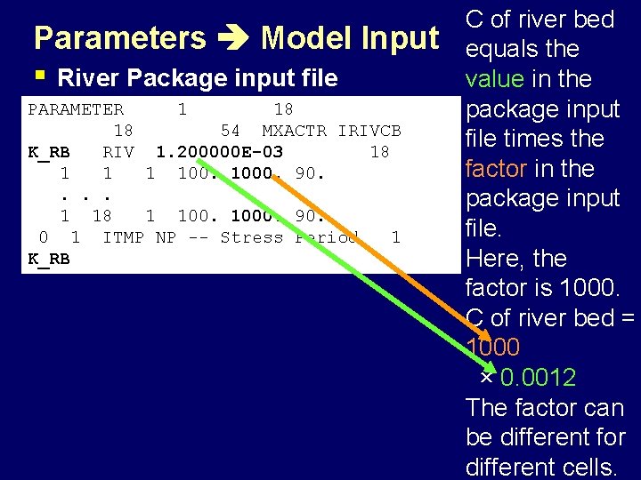
Parameters Model Input § River Package input file PARAMETER 1 18 18 54 MXACTR IRIVCB K_RB RIV 1. 200000 E-03 18 1 1000. 90. . 1 18 1 1000. 90. 0 1 ITMP NP -- Stress Period 1 K_RB C of river bed equals the value in the package input file times the factor in the package input file. Here, the factor is 1000. C of river bed = 1000 × 0. 0012 The factor can be different for different cells.

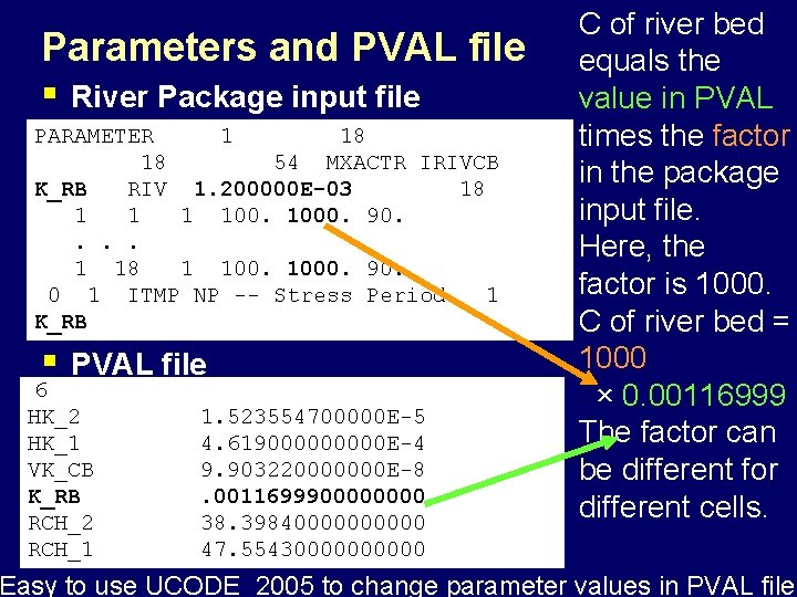
Parameters and PVAL file § River Package input file PARAMETER 1 18 18 54 MXACTR IRIVCB K_RB RIV 1. 200000 E-03 18 1 1000. 90. . 1 18 1 1000. 90. 0 1 ITMP NP -- Stress Period 1 K_RB § PVAL file 6 HK_2 HK_1 VK_CB K_RB RCH_2 RCH_1 1. 523554700000 E-5 4. 61900000 E-4 9. 903220000000 E-8. 001169990000 38. 398400000 47. 554300000 C of river bed equals the value in PVAL times the factor in the package input file. Here, the factor is 1000. C of river bed = 1000 × 0. 00116999 The factor can be different for different cells. Easy to use UCODE_2005 to change parameter values in PVAL file.

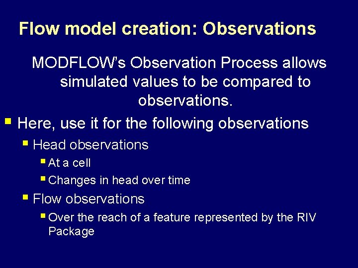
Flow model creation: Observations MODFLOW’s Observation Process allows simulated values to be compared to observations. § Here, use it for the following observations § Head observations § At a cell § Changes in head over time § Flow observations § Over the reach of a feature represented by the RIV Package

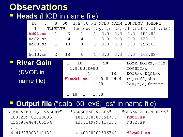
Observations § Heads (HOB in name file) 10 0 0 50 1. E+30 NH, MOBS, MAXM, IUHOBSV, HOBDRY 1. TOMULTH (below, lay, r, c, ts, roff, coff, toff, obs) hd 01. ss 1 3 1 1 0. 0 101. 80 hd 02. ss 1 4 4 1 0. 0 128. 12 hd 03. ss 1 10 9 1 0. 0 156. 68. . . hd 10. ss 2 18 6 1 0. 0 142. 02 § River Gain (RVOB in name file) § 1 18 1 50 1. 00000 E+00 1 18 flow 01. ss 1 0. 0 -4. 4 1 1. 00. . . 1 18 1 1. 00 NQxx, NQCxx, NQTx TOMULTxx NQOBxx, NQCLxx ts, toff, obs lay, r, c, factor Output file (“data 50 ex 8. _os” in name file) "SIMULATED EQUIVALENT" 100. 209701538086 126. 954444885254. . . -4. 41627883911133 "OBSERVED VALUE" 101. 800003051758 128. 119995117188 -4. 40000009536743 "OBSERVATION NAME" hd 01. ss hd 02. ss flow 01. ss

Constructing input files § § In class we will either use 00 -MFI 2005. exe or the files will be constructed already. Instructions for using 00_MFI 2005. bat are provided in class.

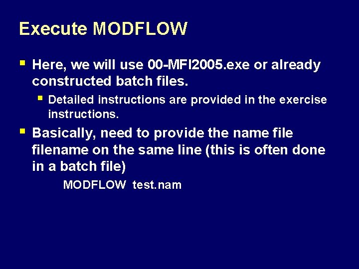
Execute MODFLOW § Here, we will use 00 -MFI 2005. exe or already constructed batch files. § Detailed instructions are provided in the exercise instructions. § Basically, need to provide the name filename on the same line (this is often done in a batch file) MODFLOW test. nam

Model results § Possible results for class problem (depends on options chosen) § Global budget (check for overall solution accuracy) § Heads at each active cell in the grid at each time step § Flows at each cell face § Simulated equivalents to observations § Often use software to visualize results. In class, use Model. Viewer

Pathline Modeling § § Advective transport. Used here as a first investigation of transport predictions Requires: § Flow solution § Porosity – to determine velocity § Starting locations § The particle tracking is calculated using MODPATH, which uses results produced by MODFLOW.