An introduction to Magnets for Accelerators Attilio Milanese

An introduction to Magnets for Accelerators Attilio Milanese John Adams Institute Accelerator Course 21 Jan. 2021

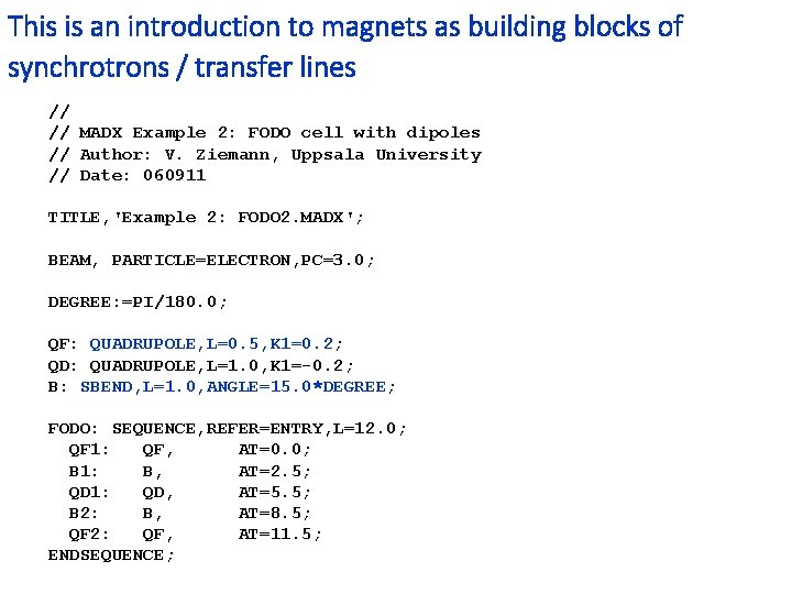
This is an introduction to magnets as building blocks of synchrotrons / transfer lines // // MADX Example 2: FODO cell with dipoles // Author: V. Ziemann, Uppsala University // Date: 060911 TITLE, 'Example 2: FODO 2. MADX'; BEAM, PARTICLE=ELECTRON, PC=3. 0; DEGREE: =PI/180. 0; QF: QUADRUPOLE, L=0. 5, K 1=0. 2; QD: QUADRUPOLE, L=1. 0, K 1=-0. 2; B: SBEND, L=1. 0, ANGLE=15. 0*DEGREE; FODO: SEQUENCE, REFER=ENTRY, L=12. 0; QF 1: QF, AT=0. 0; B 1: B, AT=2. 5; QD 1: QD, AT=5. 5; B 2: B, AT=8. 5; QF 2: QF, AT=11. 5; ENDSEQUENCE;

If you want to know more… 1. N. Marks, Magnets for Accelerators, JAI (John Adams Institute) course, Jan. 2015 2. D. Tommasini, Practical Definitions & Formulae for Normal Conducting Magnets 3. Lectures about magnets in CERN Accelerator Schools 4. Special CAS edition on magnets, Bruges, Jun. 2009 5. Lectures about magnets in JUAS (Joint Universities Accelerator School) 6. Superconducting magnets for particle accelerators in USPAS (U. S. Particle Accelerator Schools) 7. J. Tanabe, Iron Dominated Electromagnets 8. P. Campbell, Permanent Magnet Materials and their Application 9. K. -H. Mess, P. Schmüser, S. Wolff, Superconducting Accelerator Magnets 10. M. N. Wilson, Superconducting Magnets 11. A. Devred, Practical Low-Temperature Superconductors for Electromagnets 12. L. Rossi and E. Todesco, Electromagnetic design of superconducting dipoles based on sector coils

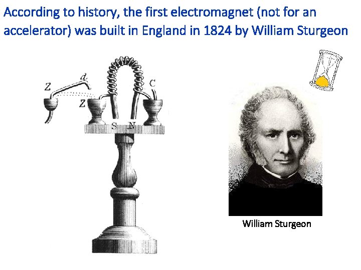
According to history, the first electromagnet (not for an accelerator) was built in England in 1824 by William Sturgeon

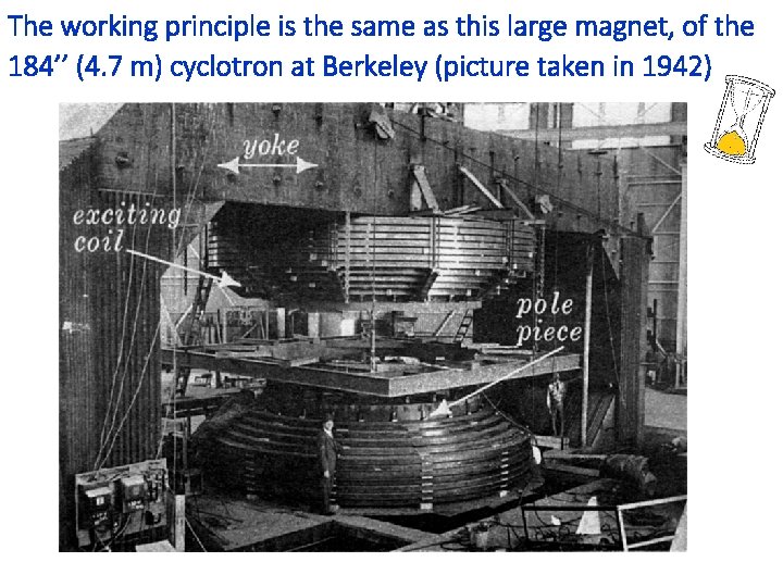
The working principle is the same as this large magnet, of the 184’’ (4. 7 m) cyclotron at Berkeley (picture taken in 1942)

This short course is organized in several blocks 1. Introduction, jargon, general concepts and formulae 2. Resistive magnets 3. Superconducting magnets 4. Tutorial with FEMM

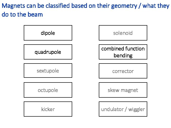
Magnets can be classified based on their geometry / what they do to the beam dipole solenoid quadrupole combined function bending sextupole corrector octupole skew magnet kicker undulator / wiggler

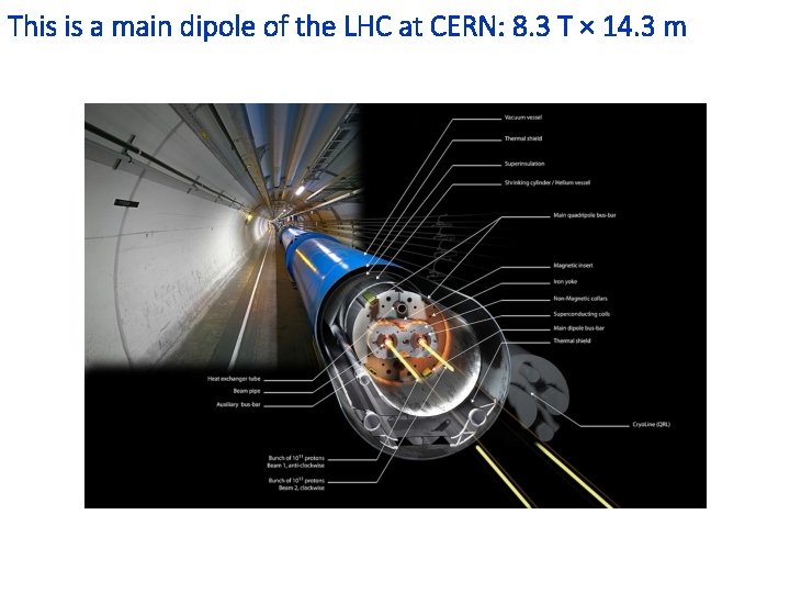
This is a main dipole of the LHC at CERN: 8. 3 T × 14. 3 m

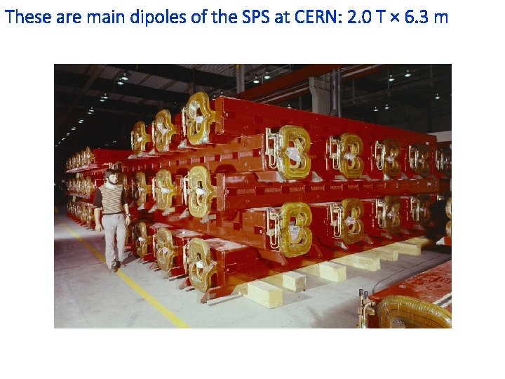
These are main dipoles of the SPS at CERN: 2. 0 T × 6. 3 m

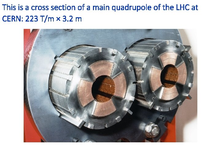
This is a cross section of a main quadrupole of the LHC at CERN: 223 T/m × 3. 2 m

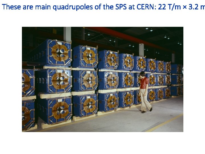
These are main quadrupoles of the SPS at CERN: 22 T/m × 3. 2 m

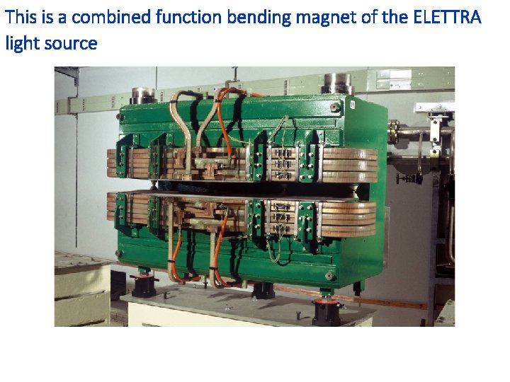
This is a combined function bending magnet of the ELETTRA light source

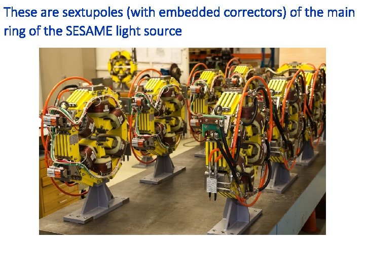
These are sextupoles (with embedded correctors) of the main ring of the SESAME light source

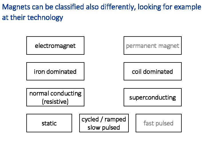
Magnets can be classified also differently, looking for example at their technology electromagnet permanent magnet iron dominated coil dominated normal conducting (resistive) superconducting static cycled / ramped slow pulsed fast pulsed

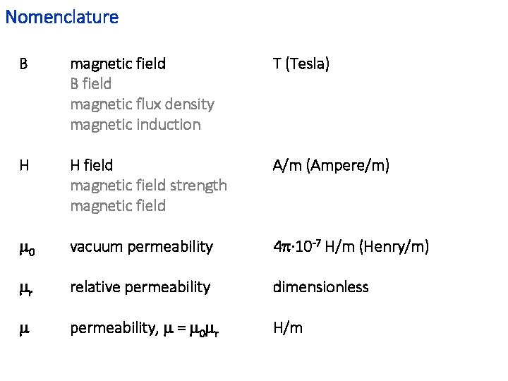
Nomenclature B magnetic field B field magnetic flux density magnetic induction T (Tesla) H H field magnetic field strength magnetic field A/m (Ampere/m) m 0 vacuum permeability 4 p∙ 10 -7 H/m (Henry/m) mr relative permeability dimensionless m permeability, m = m 0 mr H/m

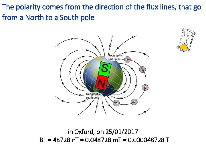
The polarity comes from the direction of the flux lines, that go from a North to a South pole in Oxford, on 25/01/2017 |B| = 48728 n. T = 0. 048728 m. T = 0. 000048728 T

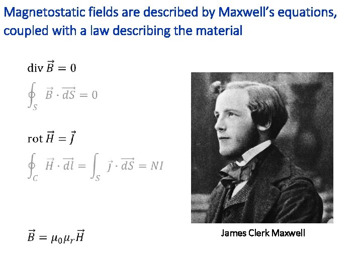
Magnetostatic fields are described by Maxwell’s equations, coupled with a law describing the material James Clerk Maxwell

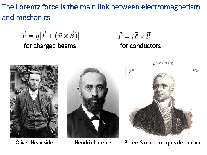
The Lorentz force is the main link between electromagnetism and mechanics for charged beams Oliver Heaviside Hendrik Lorentz for conductors Pierre-Simon, marquis de Laplace

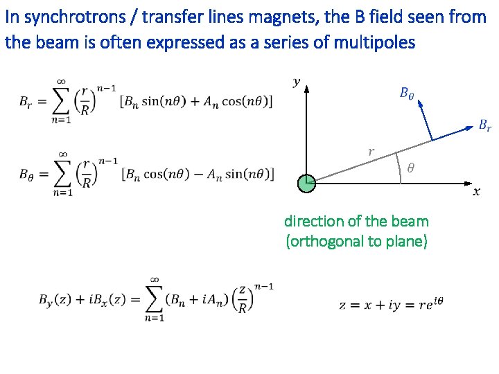
In synchrotrons / transfer lines magnets, the B field seen from the beam is often expressed as a series of multipoles direction of the beam (orthogonal to plane)

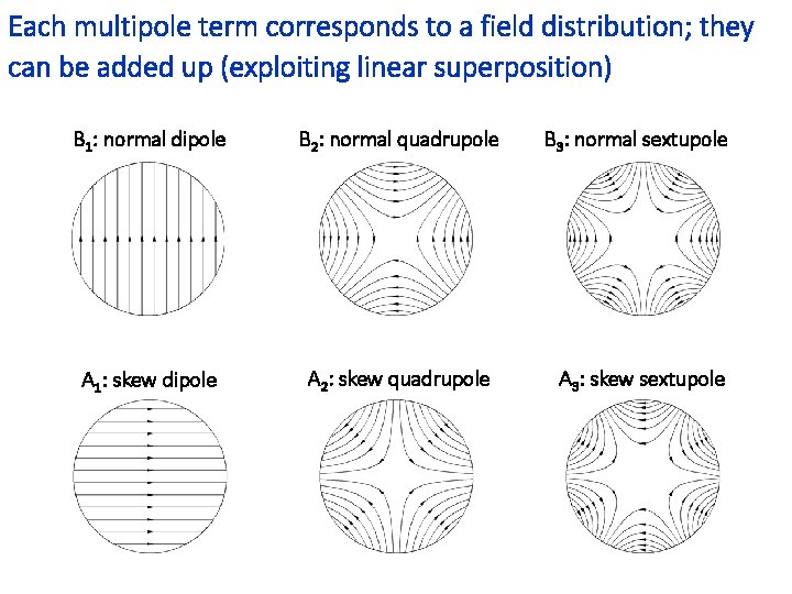
Each multipole term corresponds to a field distribution; they can be added up (exploiting linear superposition) B 1: normal dipole B 2: normal quadrupole B 3: normal sextupole A 1: skew dipole A 2: skew quadrupole A 3: skew sextupole

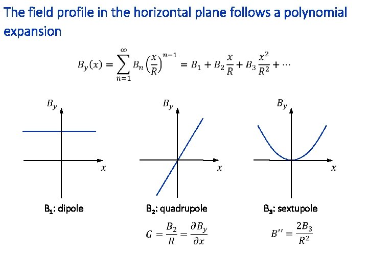
The field profile in the horizontal plane follows a polynomial expansion B 1: dipole B 2: quadrupole B 3: sextupole

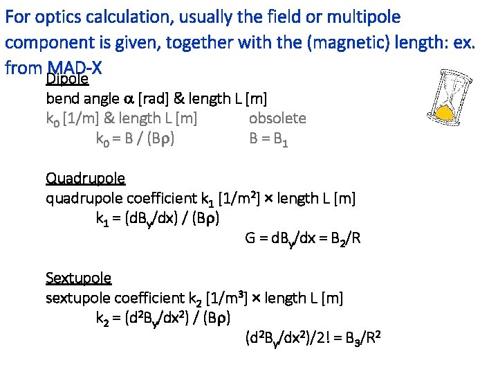
For optics calculation, usually the field or multipole component is given, together with the (magnetic) length: ex. from Dipole MAD-X bend angle a [rad] & length L [m] k 0 [1/m] & length L [m] obsolete k 0 = B / (Br) B = B 1 Quadrupole quadrupole coefficient k 1 [1/m 2] × length L [m] k 1 = (d. By/dx) / (Br) G = d. By/dx = B 2/R Sextupole sextupole coefficient k 2 [1/m 3] × length L [m] k 2 = (d 2 By/dx 2) / (Br) (d 2 By/dx 2)/2! = B 3/R 2

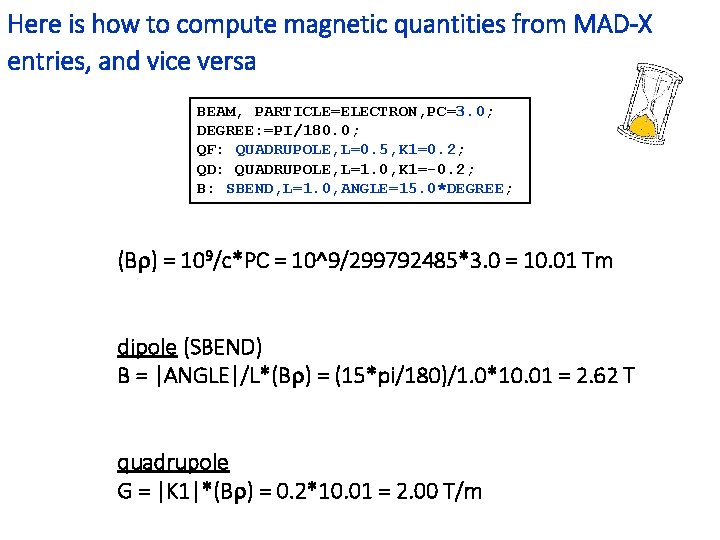
Here is how to compute magnetic quantities from MAD-X entries, and vice versa BEAM, PARTICLE=ELECTRON, PC=3. 0; DEGREE: =PI/180. 0; QF: QUADRUPOLE, L=0. 5, K 1=0. 2; QD: QUADRUPOLE, L=1. 0, K 1=-0. 2; B: SBEND, L=1. 0, ANGLE=15. 0*DEGREE; (Br) = 109/c*PC = 10^9/299792485*3. 0 = 10. 01 Tm dipole (SBEND) B = |ANGLE|/L*(Br) = (15*pi/180)/1. 0*10. 01 = 2. 62 T quadrupole G = |K 1|*(Br) = 0. 2*10. 01 = 2. 00 T/m

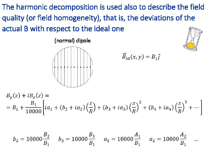
The harmonic decomposition is used also to describe the field quality (or field homogeneity), that is, the deviations of the actual B with respect to the ideal one (normal) dipole

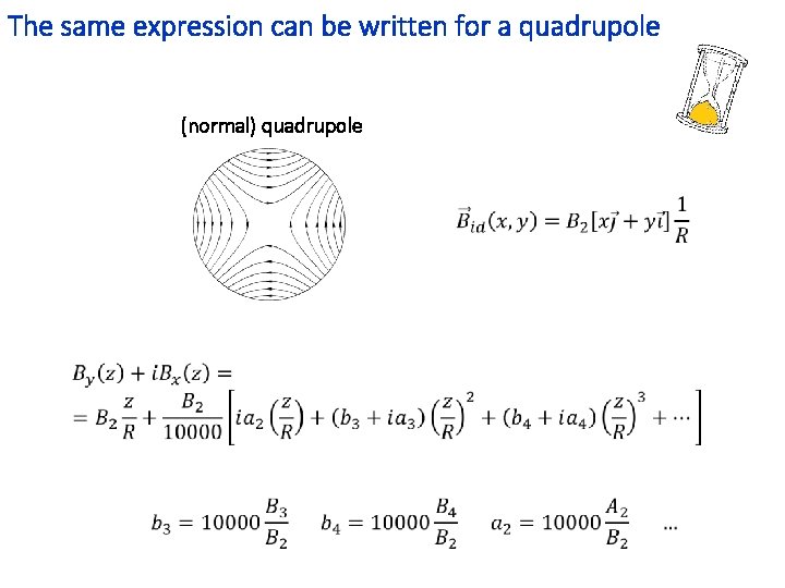
The same expression can be written for a quadrupole (normal) quadrupole

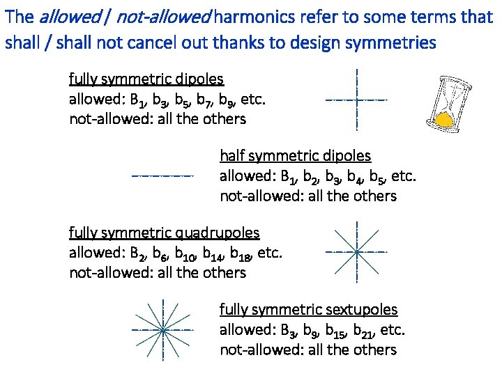
The allowed / not-allowed harmonics refer to some terms that shall / shall not cancel out thanks to design symmetries fully symmetric dipoles allowed: B 1, b 3, b 5, b 7, b 9, etc. not-allowed: all the others half symmetric dipoles allowed: B 1, b 2, b 3, b 4, b 5, etc. not-allowed: all the others fully symmetric quadrupoles allowed: B 2, b 6, b 10, b 14, b 18, etc. not-allowed: all the others fully symmetric sextupoles allowed: B 3, b 9, b 15, b 21, etc. not-allowed: all the others

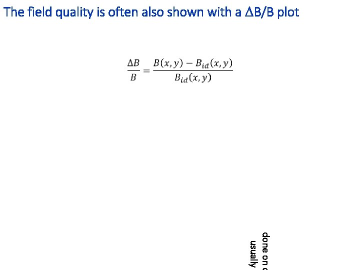
The field quality is often also shown with a DB/B plot done on o usually

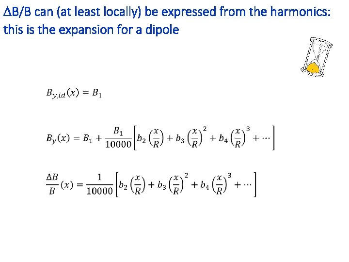
DB/B can (at least locally) be expressed from the harmonics: this is the expansion for a dipole

1. Introduction, jargon, general concepts and formulae 2. Resistive magnets 3. Superconducting magnets 4. Tutorial with FEMM

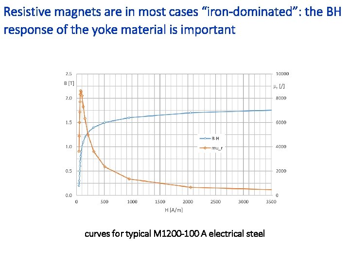
Resistive magnets are in most cases “iron-dominated”: the BH response of the yoke material is important curves for typical M 1200 -100 A electrical steel

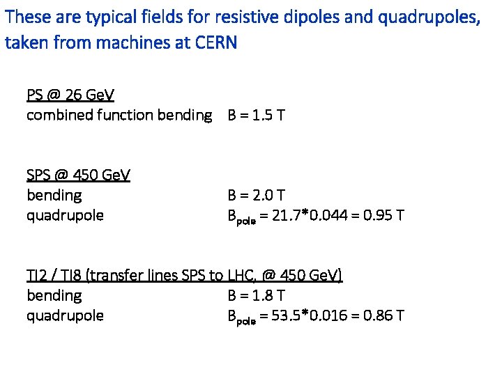
These are typical fields for resistive dipoles and quadrupoles, taken from machines at CERN PS @ 26 Ge. V combined function bending B = 1. 5 T SPS @ 450 Ge. V bending quadrupole B = 2. 0 T Bpole = 21. 7*0. 044 = 0. 95 T TI 2 / TI 8 (transfer lines SPS to LHC, @ 450 Ge. V) bending B = 1. 8 T quadrupole Bpole = 53. 5*0. 016 = 0. 86 T

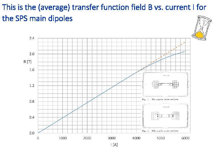
This is the (average) transfer function field B vs. current I for the SPS main dipoles

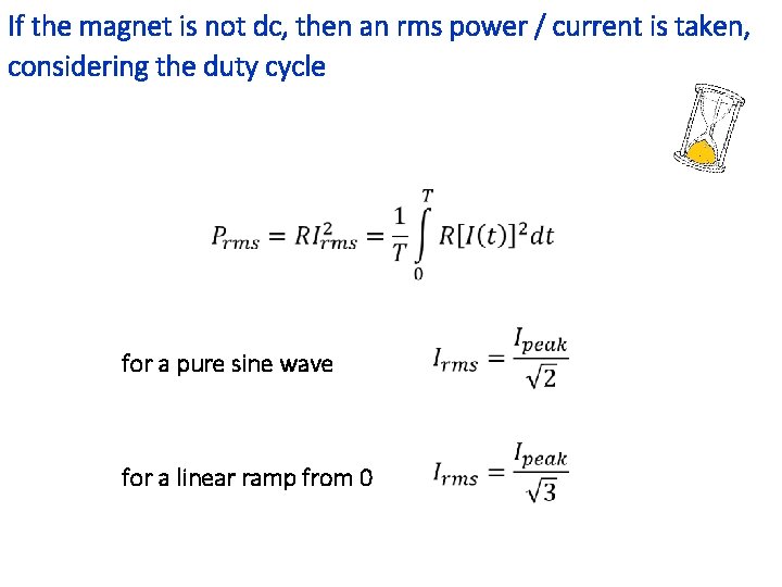
If the magnet is not dc, then an rms power / current is taken, considering the duty cycle for a pure sine wave for a linear ramp from 0

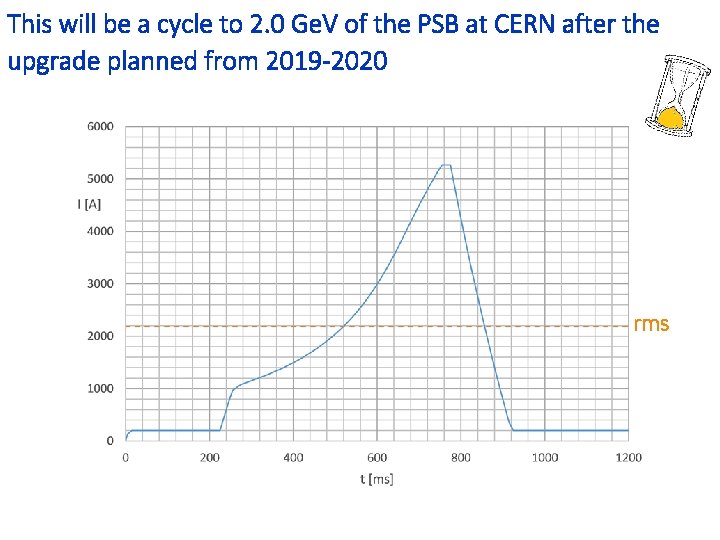
This will be a cycle to 2. 0 Ge. V of the PSB at CERN after the upgrade planned from 2019 -2020 rms

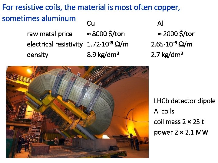
For resistive coils, the material is most often copper, sometimes aluminum Cu raw metal price ≈ 8000 $/ton electrical resistivity 1. 72∙ 10 -8 W/m density 8. 9 kg/dm 3 Al ≈ 2000 $/ton 2. 65∙ 10 -8 W/m 2. 7 kg/dm 3 LHCb detector dipole Al coils coil mass 2 × 25 t power 2 × 2. 1 MW

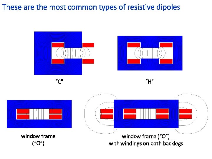
These are the most common types of resistive dipoles “C” window frame (“O”) “H” window frame (“O”) with windings on both backlegs

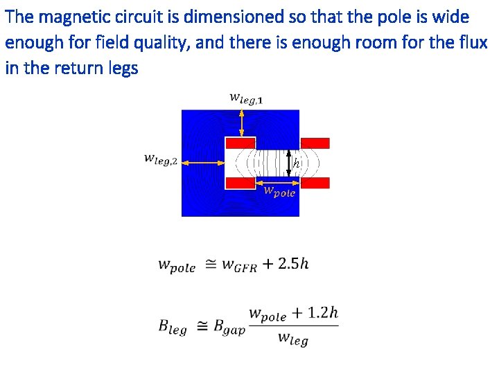
The magnetic circuit is dimensioned so that the pole is wide enough for field quality, and there is enough room for the flux in the return legs h

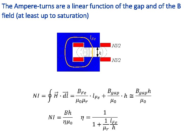
The Ampere-turns are a linear function of the gap and of the B field (at least up to saturation) NI/2 h NI/2

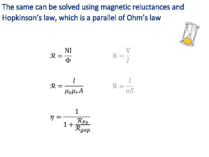
The same can be solved using magnetic reluctances and Hopkinson’s law, which is a parallel of Ohm’s law

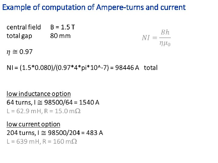
Example of computation of Ampere-turns and current

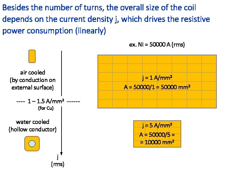
Besides the number of turns, the overall size of the coil depends on the current density j, which drives the resistive power consumption (linearly) ex. NI = 50000 A (rms) air cooled (by conduction on external surface) j = 1 A/mm 2 A = 50000/1 = 50000 mm 2 1 – 1. 5 A/mm 2 (for Cu) water cooled (hollow conductor) j (rms) j = 5 A/mm 2 A = 50000/5 = = 10000 mm 2

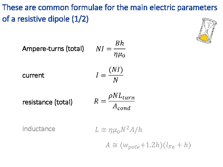
These are common formulae for the main electric parameters of a resistive dipole (1/2) Ampere-turns (total) current resistance (total) inductance

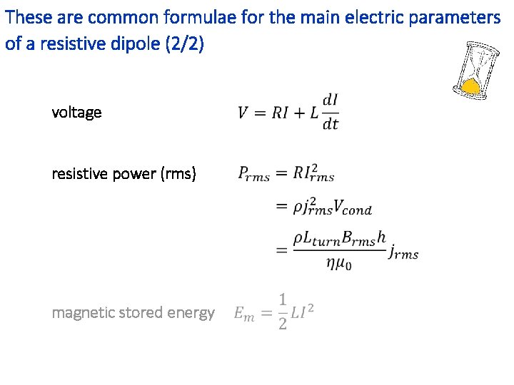
These are common formulae for the main electric parameters of a resistive dipole (2/2) voltage resistive power (rms) magnetic stored energy

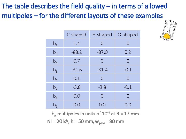
The table describes the field quality – in terms of allowed multipoles – for the different layouts of these examples C-shaped H-shaped O-shaped b 2 1. 4 0 0 b 3 -88. 2 -87. 0 0. 2 b 4 0. 7 0 0 b 5 -31. 6 -31. 4 -0. 1 b 6 0. 1 0 0 b 7 -3. 8 -0. 1 b 8 0. 0 0 0 b 9 0. 0 bn multipoles in units of 10 -4 at R = 17 mm NI = 20 k. A, h = 50 mm, wpole = 80 mm

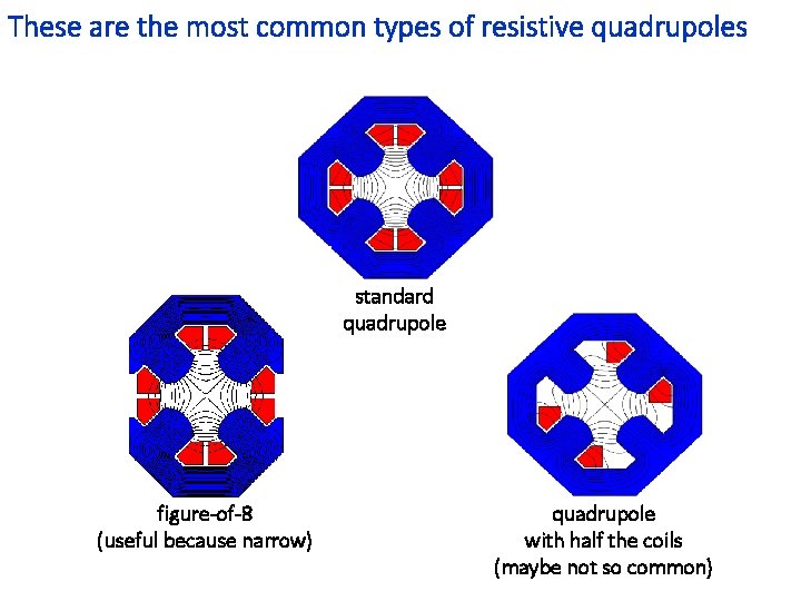
These are the most common types of resistive quadrupoles standard quadrupole figure-of-8 (useful because narrow) quadrupole with half the coils (maybe not so common)

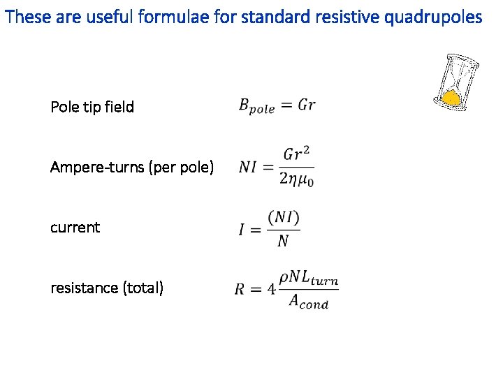
These are useful formulae for standard resistive quadrupoles Pole tip field Ampere-turns (per pole) current resistance (total)

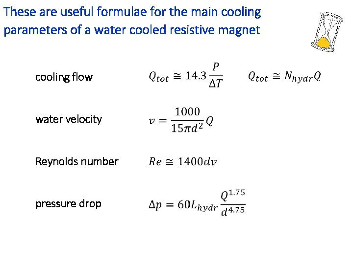
These are useful formulae for the main cooling parameters of a water cooled resistive magnet cooling flow water velocity Reynolds number pressure drop

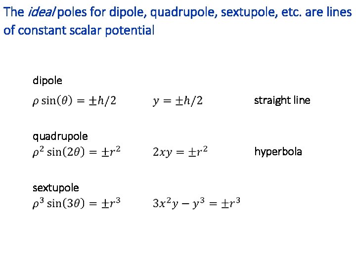
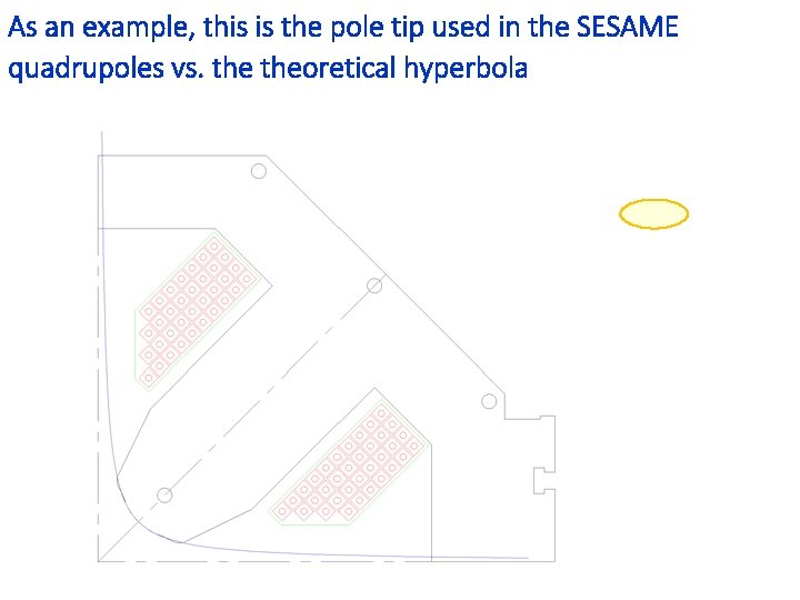
The ideal poles for dipole, quadrupole, sextupole, etc. are lines of constant scalar potential dipole straight line quadrupole hyperbola sextupole

As an example, this is the pole tip used in the SESAME quadrupoles vs. theoretical hyperbola

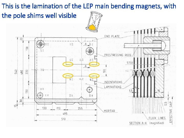
This is the lamination of the LEP main bending magnets, with the pole shims well visible

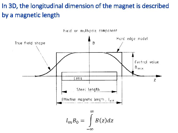
In 3 D, the longitudinal dimension of the magnet is described by a magnetic length

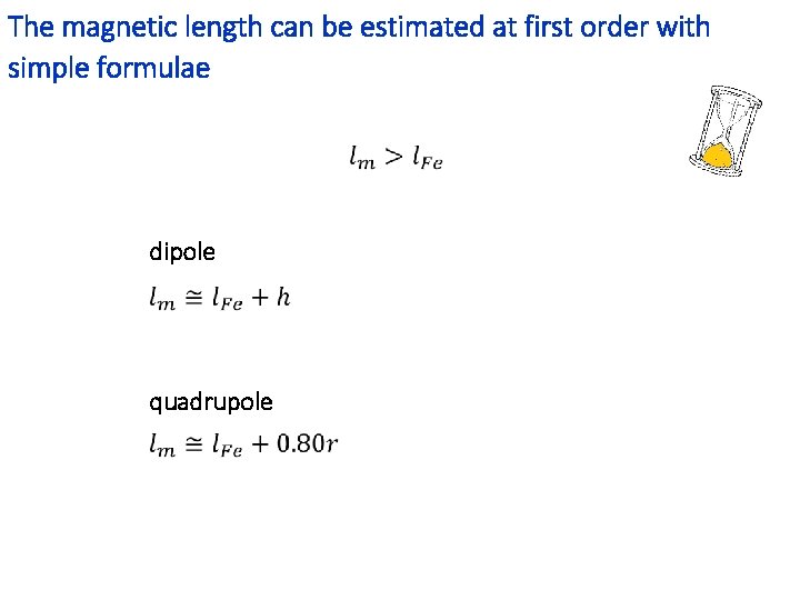
The magnetic length can be estimated at first order with simple formulae dipole quadrupole

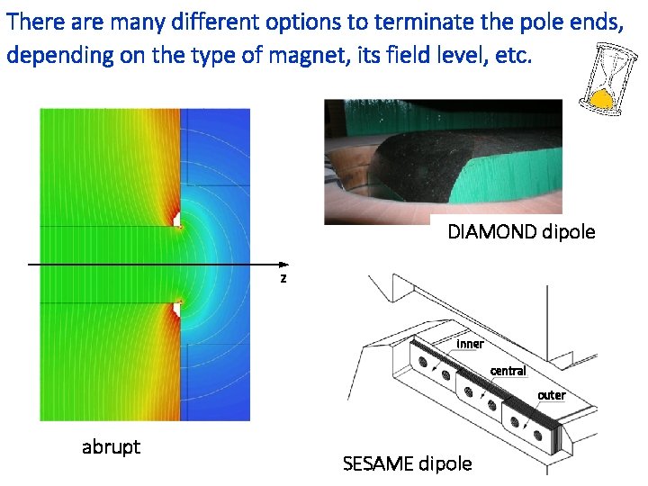
There are many different options to terminate the pole ends, depending on the type of magnet, its field level, etc. DIAMOND dipole z inner central outer abrupt SESAME dipole

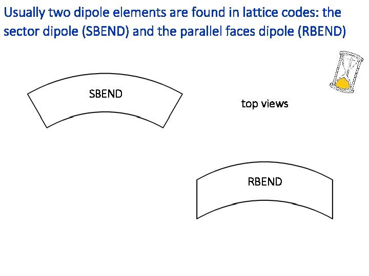
Usually two dipole elements are found in lattice codes: the sector dipole (SBEND) and the parallel faces dipole (RBEND) SBEND top views RBEND

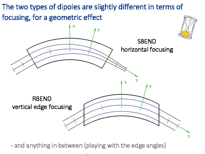
The two types of dipoles are slightly different in terms of focusing, for a geometric effect SBEND horizontal focusing RBEND vertical edge focusing - and anything in between (playing with the edge angles)

1. Introduction, jargon, general concepts and formulae 2. Resistive magnets 3. Superconducting magnets (thanks to Luca Bottura for the material of many slides) 4. Tutorial with FEMM

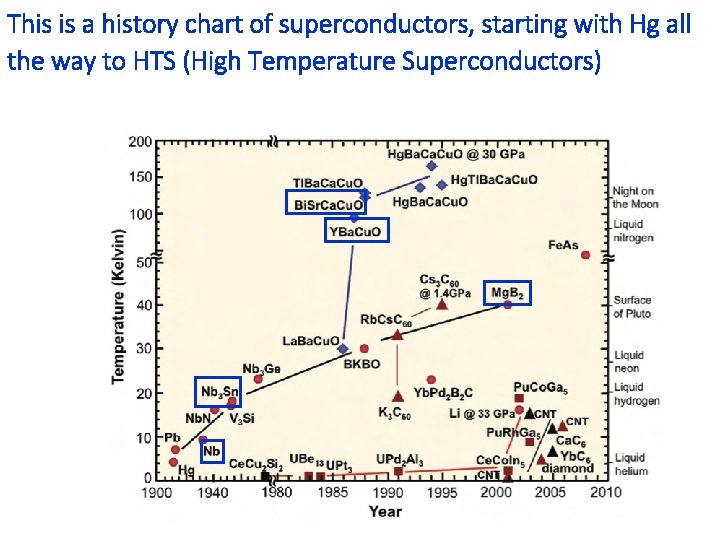
This is a history chart of superconductors, starting with Hg all the way to HTS (High Temperature Superconductors)

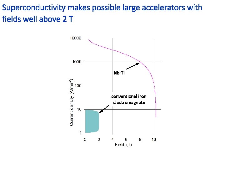
Superconductivity makes possible large accelerators with fields well above 2 T Nb-Ti conventional iron electromagnets

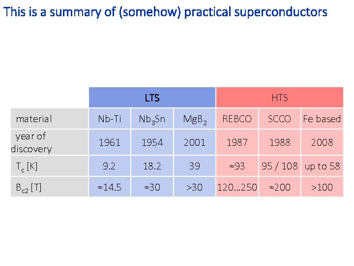
This is a summary of (somehow) practical superconductors LTS HTS material Nb-Ti Nb 3 Sn Mg. B 2 REBCO SCCO Fe based year of discovery 1961 1954 2001 1987 1988 2008 Tc [K] 9. 2 18. 2 39 ≈93 Bc 2 [T] ≈14. 5 ≈30 >30 120… 250 95 / 108 up to 58 ≈200 >100

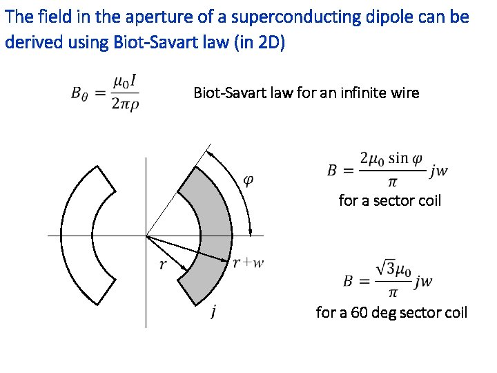
The field in the aperture of a superconducting dipole can be derived using Biot-Savart law (in 2 D) Biot-Savart law for an infinite wire for a sector coil for a 60 deg sector coil

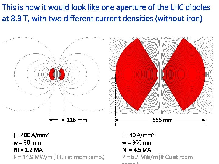
This is how it would look like one aperture of the LHC dipoles at 8. 3 T, with two different current densities (without iron) 116 mm j = 400 A/mm 2 w = 30 mm NI = 1. 2 MA P = 14. 9 MW/m (if Cu at room temp. ) 656 mm j = 40 A/mm 2 w = 300 mm NI = 4. 5 MA P = 6. 2 MW/m (if Cu at room

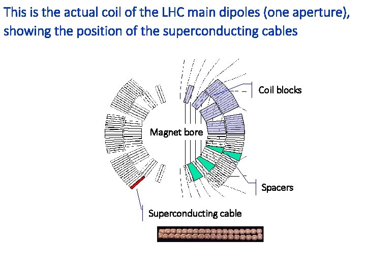
This is the actual coil of the LHC main dipoles (one aperture), showing the position of the superconducting cables Coil blocks Magnet bore Spacers Superconducting cable

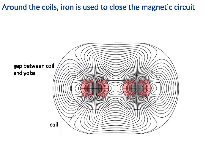
Around the coils, iron is used to close the magnetic circuit gap between coil and yoke coil

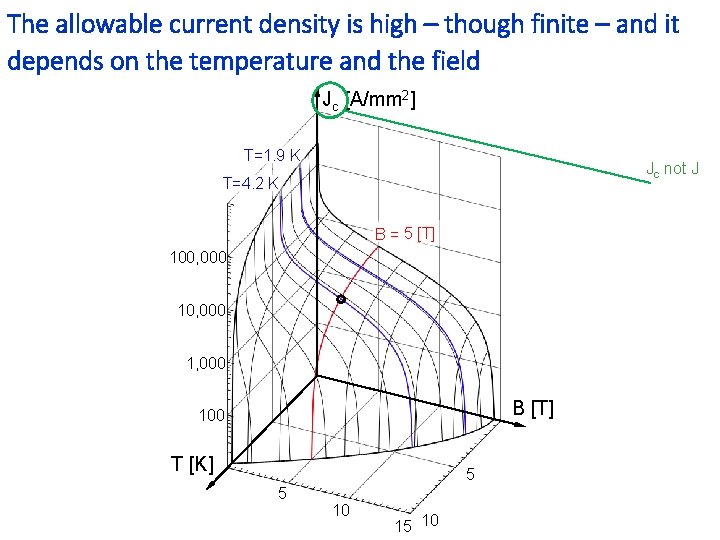
The allowable current density is high – though finite – and it depends on the temperature and the field Jc [A/mm 2] T=1. 9 K Jc not J T=4. 2 K B = 5 [T] 100, 000 1, 000 B [T] 100 T [K] 5 5 10 15 10

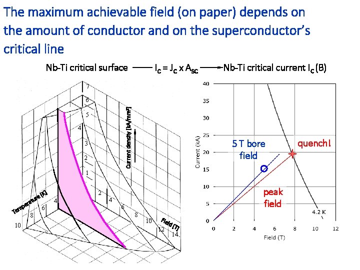
The maximum achievable field (on paper) depends on the amount of conductor and on the superconductor’s critical line Nb-Ti critical surface IC = JC x ASC Nb-Ti critical current IC (B) 7 Current density [k. A/mm 2] 6 5 4 3 2 5 T bore field 1 p em e tur a r e T 10 8 [K] 6 4 2 peak field 2 4 6 8 10 Fie 12 ld [ T] 14 quench!

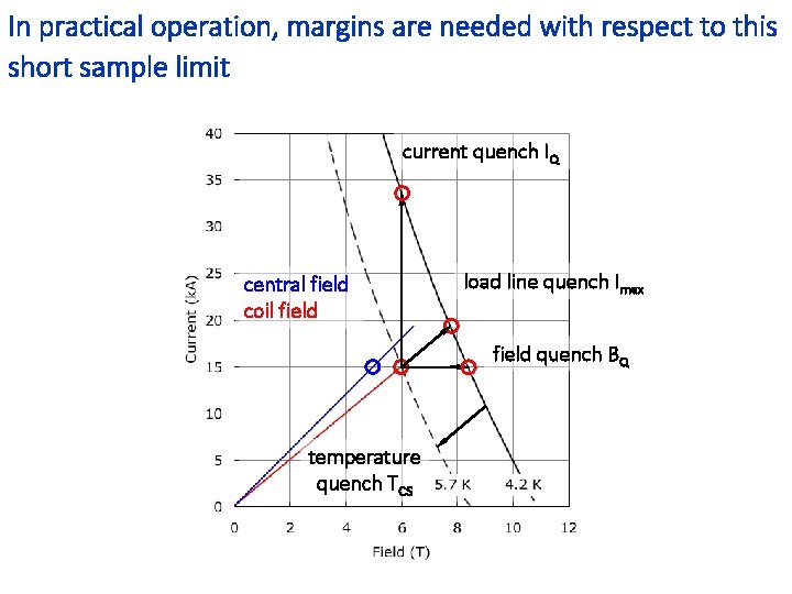
In practical operation, margins are needed with respect to this short sample limit current quench IQ central field coil field load line quench Imax field quench BQ temperature quench TCS

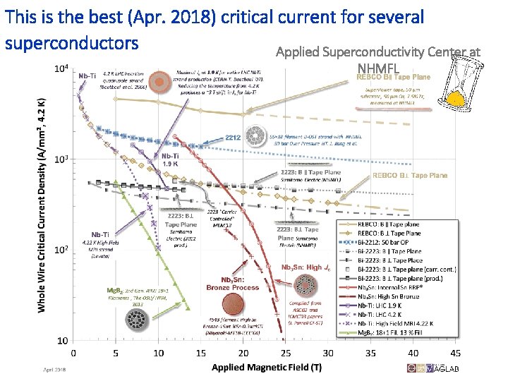
This is the best (Apr. 2018) critical current for several superconductors Applied Superconductivity Center at NHMFL

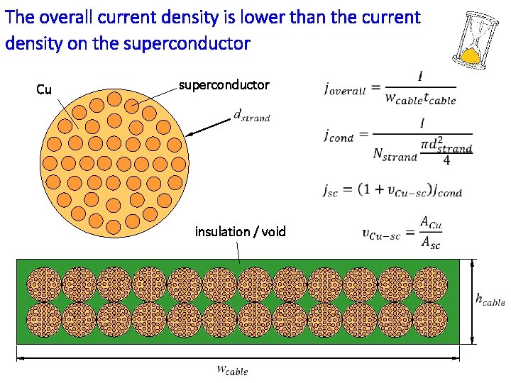
The overall current density is lower than the current density on the superconductor Cu superconductor insulation / void

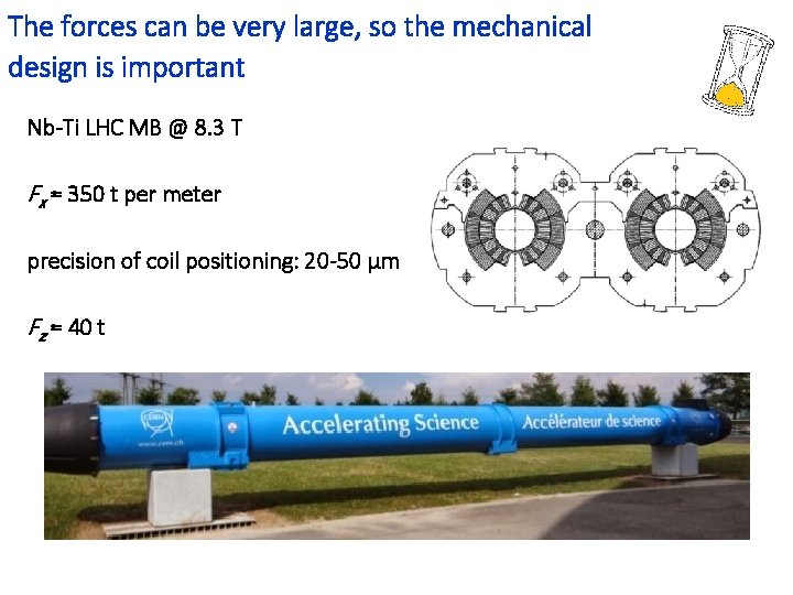
The forces can be very large, so the mechanical design is important Nb-Ti LHC MB @ 8. 3 T Fx ≈ 350 t per meter precision of coil positioning: 20 -50 μm Fz ≈ 40 t

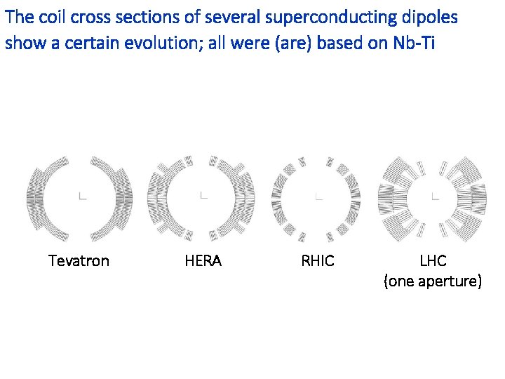
The coil cross sections of several superconducting dipoles show a certain evolution; all were (are) based on Nb-Ti Tevatron HERA RHIC LHC (one aperture)

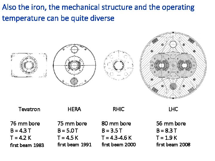
Also the iron, the mechanical structure and the operating temperature can be quite diverse Tevatron 76 mm bore B = 4. 3 T T = 4. 2 K first beam 1983 HERA 75 mm bore B = 5. 0 T T = 4. 5 K first beam 1991 RHIC 80 mm bore B = 3. 5 T T = 4. 3 -4. 6 K first beam 2000 LHC 56 mm bore B = 8. 3 T T = 1. 9 K first beam 2008

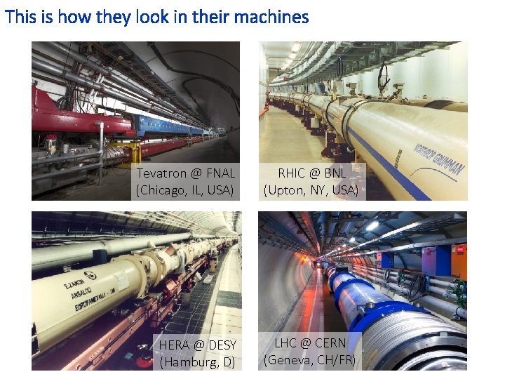
This is how they look in their machines Tevatron @ FNAL (Chicago, IL, USA) RHIC @ BNL (Upton, NY, USA) HERA @ DESY (Hamburg, D) LHC @ CERN (Geneva, CH/FR)

1. Introduction, jargon, general concepts and formulae 2. Resistive magnets 3. Superconducting magnets 4. Tutorial with FEMM As an example, we will do a 2 D model of a resistive dipole for HIE-ISOLDE

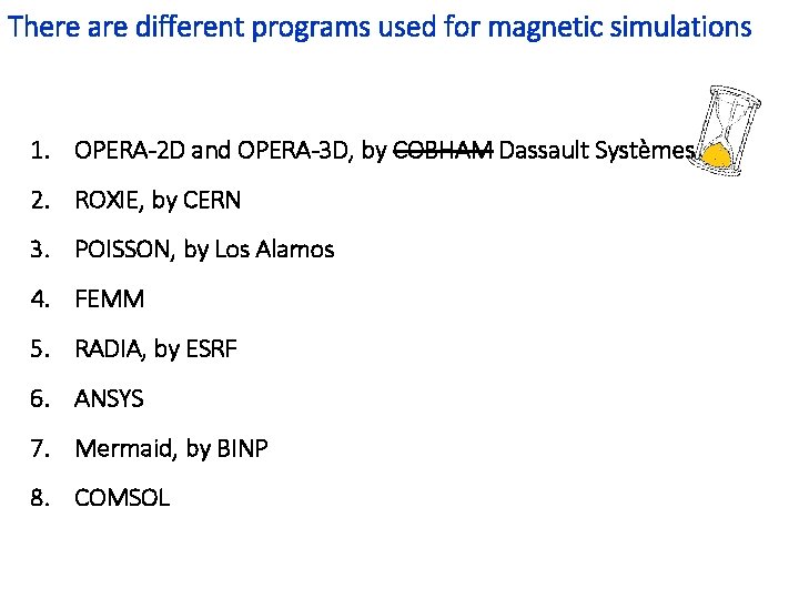
There are different programs used for magnetic simulations 1. OPERA-2 D and OPERA-3 D, by COBHAM Dassault Systèmes 2. ROXIE, by CERN 3. POISSON, by Los Alamos 4. FEMM 5. RADIA, by ESRF 6. ANSYS 7. Mermaid, by BINP 8. COMSOL

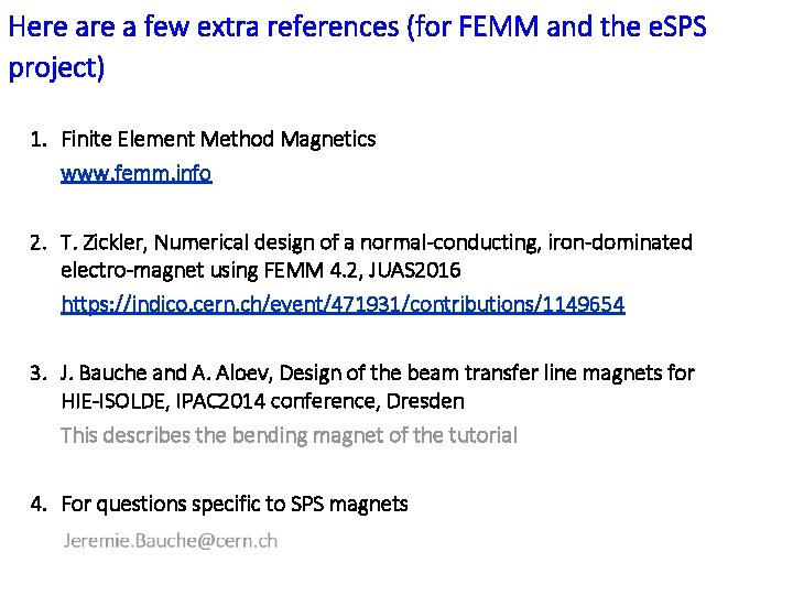
Here a few extra references (for FEMM and the e. SPS project) 1. Finite Element Method Magnetics www. femm. info 2. T. Zickler, Numerical design of a normal-conducting, iron-dominated electro-magnet using FEMM 4. 2, JUAS 2016 https: //indico. cern. ch/event/471931/contributions/1149654 3. J. Bauche and A. Aloev, Design of the beam transfer line magnets for HIE-ISOLDE, IPAC 2014 conference, Dresden This describes the bending magnet of the tutorial 4. For questions specific to SPS magnets

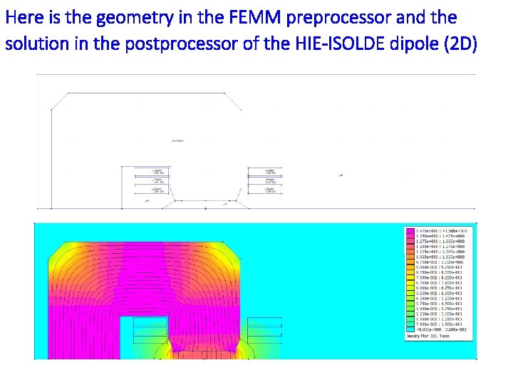
Here is the geometry in the FEMM preprocessor and the solution in the postprocessor of the HIE-ISOLDE dipole (2 D)

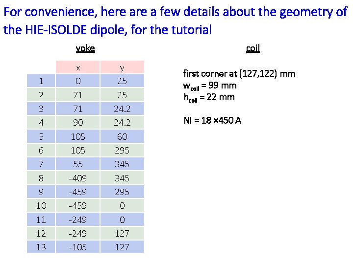
For convenience, here a few details about the geometry of the HIE-ISOLDE dipole, for the tutorial yoke 1 2 3 4 5 6 7 8 9 10 11 12 13 x 0 71 71 90 105 55 -409 -459 -249 -105 coil y 25 25 24. 2 60 295 345 295 0 0 127 first corner at (127, 122) mm wcoil = 99 mm hcoil = 22 mm NI = 18 × 450 A

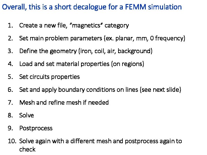
Overall, this is a short decalogue for a FEMM simulation 1. Create a new file, “magnetics” category 2. Set main problem parameters (ex. planar, mm, 0 frequency) 3. Define the geometry (iron, coil, air, background) 4. Load and set material properties (on regions) 5. Set circuits properties 6. Set and apply boundary conditions on lines (see next slide) 7. Mesh and refine mesh if needed 8. Solve 9. Postprocess 10. Solve again with a different mesh and postprocess again to check

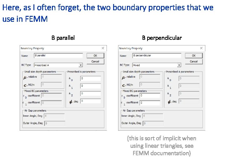
Here, as I often forget, the two boundary properties that we use in FEMM B parallel B perpendicular (this is sort of implicit when using linear triangles, see FEMM documentation)

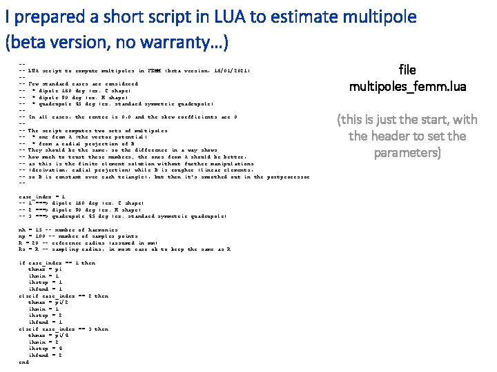
I prepared a short script in LUA to estimate multipole (beta version, no warranty…) ---------- LUA script to compute multipoles in FEMM (beta version, 16/01/2021) Few standard cases are considered: * dipole 180 deg (ex. C shape) * dipole 90 deg (ex. H shape) * quadrupole 45 deg (ex. standard symmetric quadrupole) In all cases, the center is 0, 0 and the skew coefficients are 0 The script computes two sets of multipoles: * one from A (the vector potential) * from a radial projection of B They should be the same, so the difference in a way shows how much to trust these numbers; the ones from A should be better, as this is the finite element solution without further manipulations (derivation, radial projection) while B is rougher (linear elements, so B is constant over each triangle), but then it's smoothed out in the postprocessor case_index = 1 -- 1 ===> dipole 180 deg (ex. C shape) -- 2 ===> dipole 90 deg (ex. H shape) -- 3 ===> quadrupole 45 deg (ex. standard symmetric quadrupole) nh = 15 -- number of harmonics np = 100 -- number of samples points R = 20 -- reference radius (assumed in mm) Rs = R -- sampling radius, in most case ok to keep the same as R if case_index == 1 then thmax = pi ihmin = 1 ihstep = 1 ihfund = 1 elseif case_index == 2 then thmax = pi/2 ihmin = 1 ihstep = 2 ihfund = 1 elseif case_index == 3 then thmax = pi/4 ihmin = 2 ihstep = 4 ihfund = 2 end file multipoles_femm. lua (this is just the start, with the header to set the parameters)