An Introduction to IonOptics Series of Five Lectures

An Introduction to Ion-Optics Series of Five Lectures JINA, University of Notre Dame Sept. 30 – Dec. 9, 2005 Georg P. Berg 1

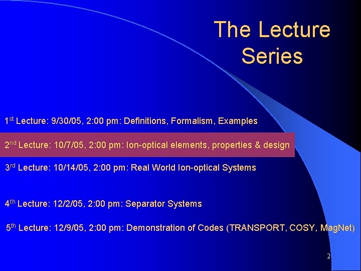
The Lecture Series 1 st Lecture: 9/30/05, 2: 00 pm: Definitions, Formalism, Examples 2 nd Lecture: 10/7/05, 2: 00 pm: Ion-optical elements, properties & design 3 rd Lecture: 10/14/05, 2: 00 pm: Real World Ion-optical Systems 4 th Lecture: 12/2/05, 2: 00 pm: Separator Systems 5 th Lecture: 12/9/05, 2: 00 pm: Demonstration of Codes (TRANSPORT, COSY, Mag. Net) 2

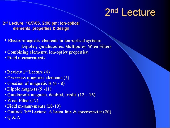
2 nd Lecture: 10/7/05, 2: 00 pm: Ion-optical elements, properties & design • Electro-magnetic elements in ion-optical systems Dipoles, Quadrupoles, Multipoles, Wien Filters • Combining elements, ion-optics properties • Field measurements • Review 1 st Lecture (4) • Overview magnetic elements (5) • Creation of magnetic B (6 - 8) • Dipole magnets (9 -11) • Quadrupole magnets, doublet, triplet (12 – 16) • Wien Filter (17) • Field measurements (18 -19) • Outlook 3 rrd Lecture: A beam line & spectrometer (20) • Q&A 3

Review 1 st Lecture (1) Lorentz Force: TRANSPORT of Ray X 0 Xn = R X 0 (3) using Matrix R R = Rn Rn-1 … R 0 (4) TRANSPORT of s Matrix (Phase space ellipsoid) Beam emittance: s 11 s 22 - (s 12) 2 e = Ö`````` s 1 = Rs 0 RT (10) (5) Taylor expansion, higher orders, solving the equation of motion, diagnostics, examples 4

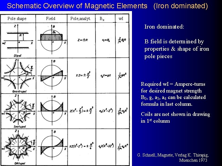
Schematic Overview of Magnetic Elements (Iron dominated) Pole shape Field Pole, analyt. Bx w. I Iron dominated: B field is determined by properties & shape of iron pole pieces Required w. I = Ampere-turns for desired magnet strength B 0, g, a 3, a 4 can be calculated formula in last column. Coils are not shown in drawing in 1 st colunm G. Schnell, Magnete, Verlag K. Thiemig, 5 Muenchen 1973

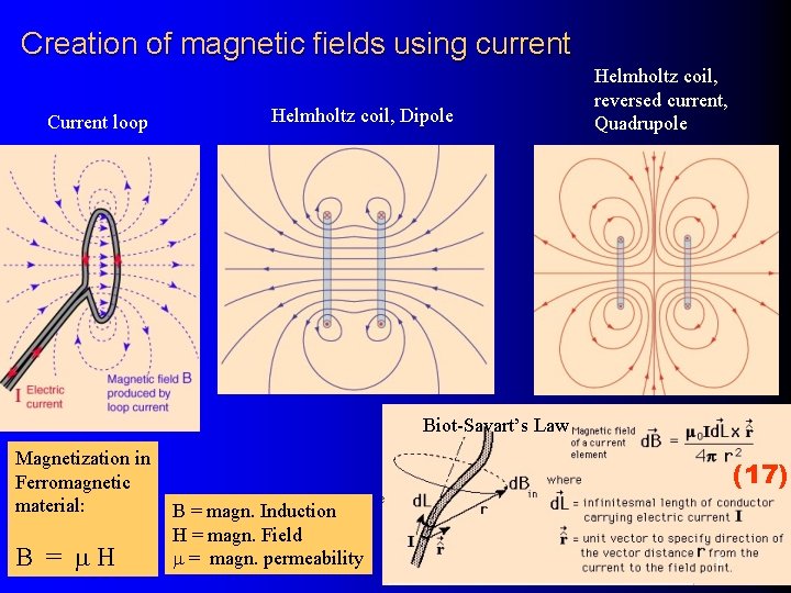
Creation of magnetic fields using current Current loop Helmholtz coil, Dipole Helmholtz coil, reversed current, Quadrupole Biot-Savart’s Law Magnetization in Ferromagnetic material: B = m. H (17) B = magn. Induction H = magn. Field m = magn. permeability 6

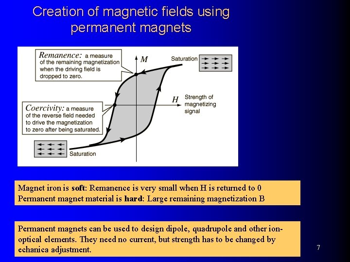
Creation of magnetic fields using permanent magnets Magnet iron is soft: Remanence is very small when H is returned to 0 Permanent magnet material is hard: Large remaining magnetization B Permanent magnets can be used to design dipole, quadrupole and other ionoptical elements. They need no current, but strength has to be changed by echanica adjustment. 7

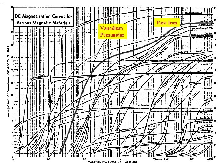
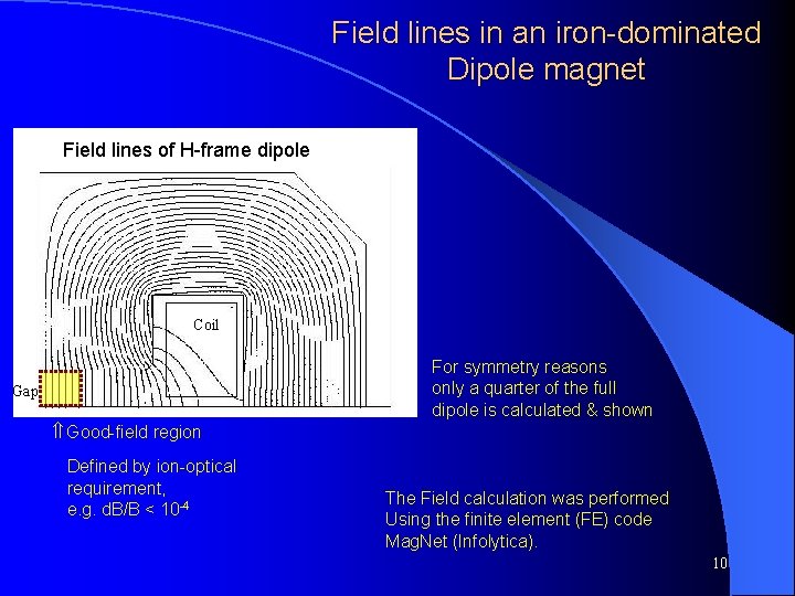
Magnetization Curves Vanadium Permandur Pure Iron Field lines of H-frame dipole 8

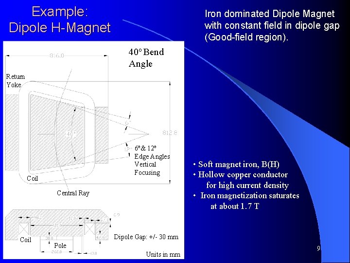
Example: Dipole H-Magnet Iron dominated Dipole Magnet with constant field in dipole gap (Good-field region). 40 o Bend Angle Return Yoke 6 o& 12 o Edge Angles Vertical Focusing Coil Central Ray Coil • Soft magnet iron, B(H) • Hollow copper conductor for high current density • Iron magnetization saturates at about 1. 7 T Dipole Gap: +/- 30 mm Pole Units in mm 9

Field lines in an iron-dominated Dipole magnet Field lines of H-frame dipole Coil For symmetry reasons only a quarter of the full dipole is calculated & shown Gap Ý Good-field region Defined by ion-optical requirement, e. g. d. B/B < 10 -4 The Field calculation was performed Using the finite element (FE) code Mag. Net (Infolytica). 10

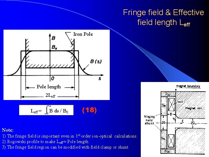
Fringe field & Effective field length Leff Iron Pole length 2 Leff = B ds / B 0 (18) Note: 1) The fringe field is important even in 1 st order ion-optical calculations. 2) Rogowski profile to make Leff = Pole length. 3) The fringe field region can be modified with field clamp or shunt. 11

Current in & out of drawing plane Standard Quadrupole y out Pole Piece Return Yoke in N S in S N in Coils in x out Note: Magnet is Iron/Current configuration with field as needed in ion-optical design. 2 d/3 d finite elements codes solving POISSON equation are well established 12

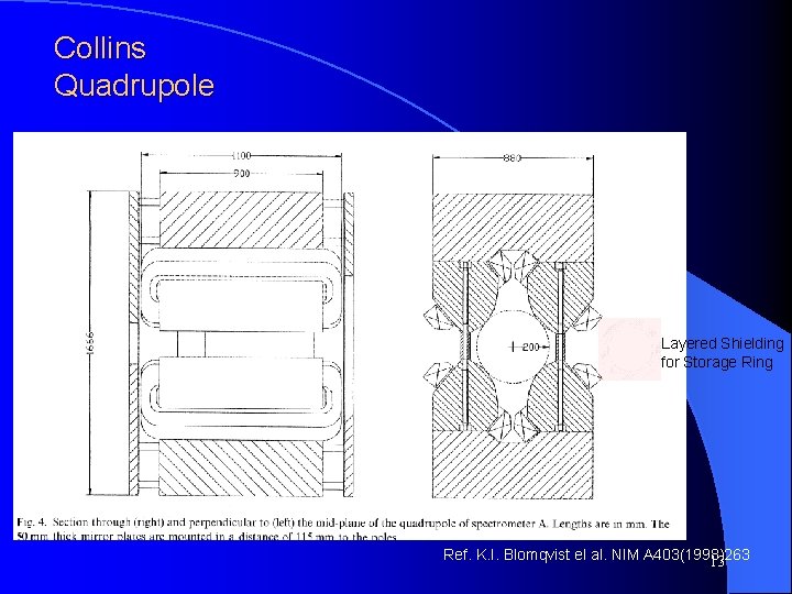
Collins Quadrupole Layered Shielding for Storage Ring Ref. K. I. Blomqvist el al. NIM A 403(1998)263 13

Forces on ions ( quadrupole) Quadrupole Hexapole Octopole ß Ü Þ Ý Horizontally defocusing quadrupole for ions along – z axis into the drawing plane. See Forces ÝÜßÞ in direction v x B A focusing quadrupole is obtained by a 90 o rotation around the z axis 14

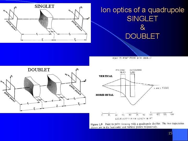
SINGLET Ion optics of a quadrupole SINGLET & DOUBLET VERTICAL HORIZONTAL 15

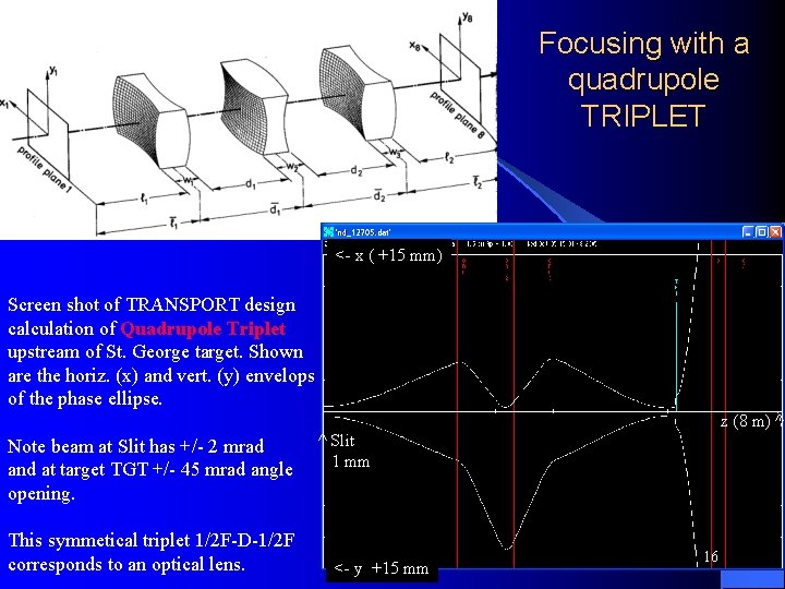
Focusing with a quadrupole TRIPLET <- x ( +15 mm) Screen shot of TRANSPORT design calculation of Quadrupole Triplet upstream of St. George target. Shown are the horiz. (x) and vert. (y) envelops of the phase ellipse. z (8 m) ^ Note beam at Slit has +/- 2 mrad and at target TGT +/- 45 mrad angle opening. This symmetical triplet 1/2 F-D-1/2 F corresponds to an optical lens. ^ Slit 1 mm <- y +15 mm 16

(1) F=0 v = E/B when q. E = qv x B with E ^ B The Wien Filter with E ^ B (19) Design study of Wien Filter for St. George Electrostatic system of Danfysik Wien Filter Units in mm Gradient of E Field lines 1, 813 k. V/mm B Field lines 0. 3 T 17

Hall Probe RH Hall Effect: UH = ¾¾ BI d (20) Lorentz force ev x B on electrons with velocity v that constitute the current I RH = Hall constant, material property Remarks: • Precision down to ~ 2 10 -4 • Needs temperature calibration • Probe area down to 1 mm by 1 mm • Average signal in gradient field (good for quadrupole and fringe field measurement) 18

Nuclear spin precesses in external field B With Larmor frequency f. L = 2 m ¾ B h NMR Probe (21) m = p, d magn. Moment h = Planck constant Nucleus with spin f. L (proton)/B = 42. 58 MHz/T f. L (deuteron)/B = 6. 538 MHz/T Fig. 1 Principle of measurement: Small (e. g. water probe), low frequency wobble coil B + B~ , tuneable HF field B» (Fig. 1) with frequency ft , observe Larmor resonance on Oscilloscope (Fig. 2). When signal a & b coincide the tuneable frequence ft = f. L • Precision ~ 10 -5 • Temperature independent • Needs constant B in probe ( 5 x 5 mm) to see signal! Fig. 2 19

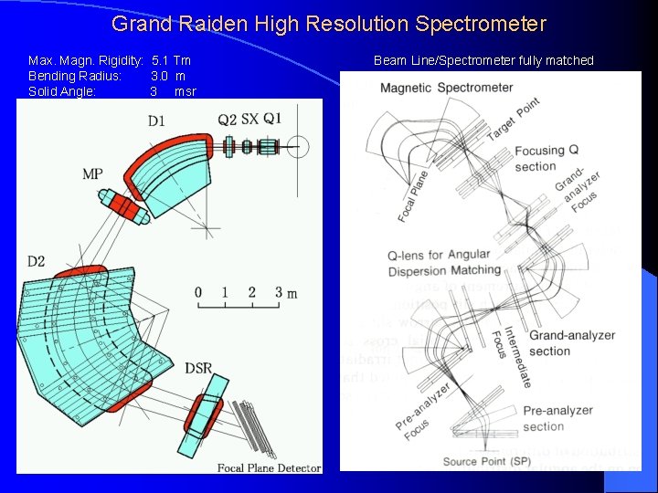
Grand Raiden High Resolution Spectrometer Max. Magn. Rigidity: 5. 1 Tm Bending Radius: 3. 0 m Solid Angle: 3 msr Beam Line/Spectrometer fully matched 20

End Lecture 2 21