An Introduction to Independent Component Analysis ICA The

An Introduction to Independent Component Analysis (ICA) 吳育德 陽明大學放射醫學科學研究所 台北榮總整合性腦功能實驗室

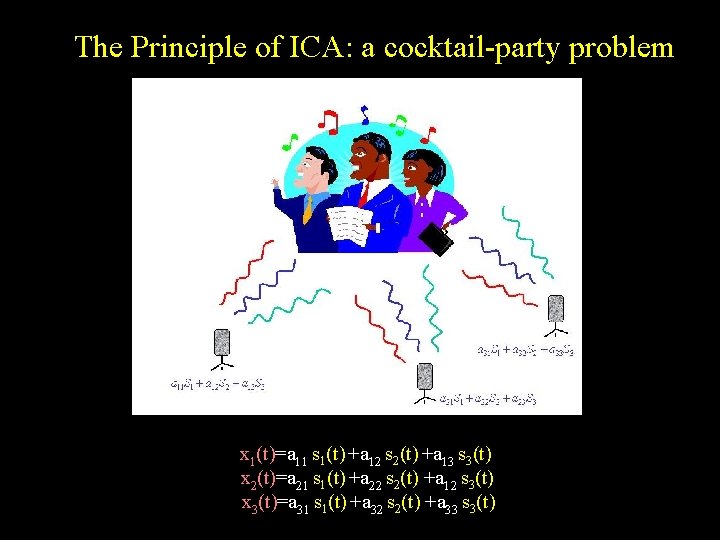
The Principle of ICA: a cocktail-party problem x 1(t)=a 11 s 1(t) +a 12 s 2(t) +a 13 s 3(t) x 2(t)=a 21 s 1(t) +a 22 s 2(t) +a 12 s 3(t) x 3(t)=a 31 s 1(t) +a 32 s 2(t) +a 33 s 3(t)

Independent Component Analysis Reference : A. Hyvärinen, J. Karhunen, E. Oja (2001) John Wiley & Sons. Independent Component Analysis

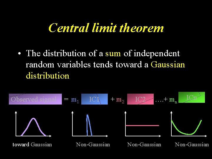
Central limit theorem • The distribution of a sum of independent random variables tends toward a Gaussian distribution Observed signal toward Gaussian = m 1 IC 1 Non-Gaussian + m 2 IC 2 …. + mn Non-Gaussian ICn Non-Gaussian

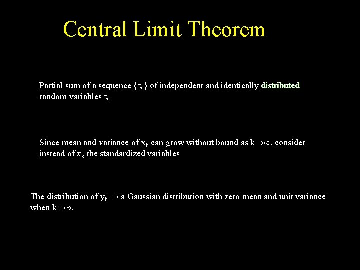
Central Limit Theorem Partial sum of a sequence {zi} of independent and identically distributed random variables zi Since mean and variance of xk can grow without bound as k , consider instead of xk the standardized variables The distribution of yk a Gaussian distribution with zero mean and unit variance when k .

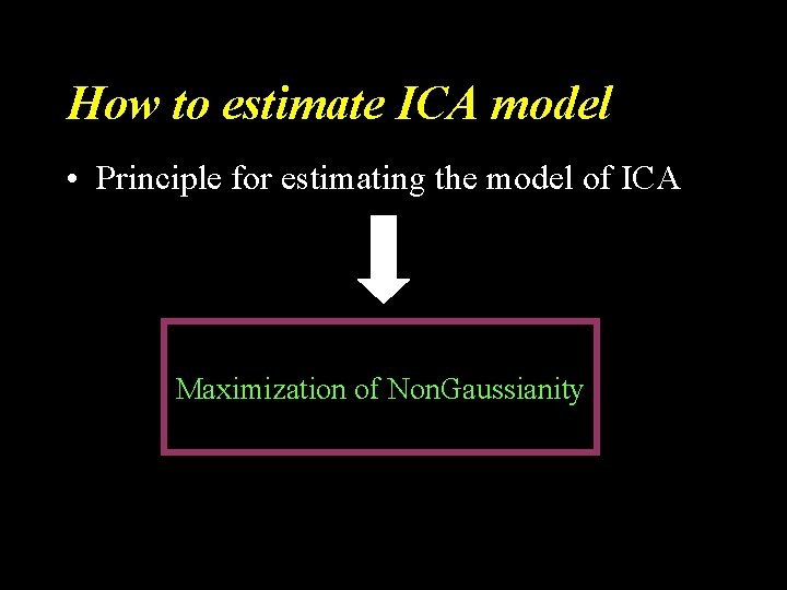
How to estimate ICA model • Principle for estimating the model of ICA Maximization of Non. Gaussianity

Measures for Non. Gaussianity • Kurtosis : E{(x- )4}-3*[E{(x- )2}] 2 Super-Gaussian kurtosis > 0 kurt(x 1+x 2)= kurt(x 1) + kurt(x 2) kurt( x 1) = 4 kurt(x 1) Gaussian kurtosis = 0 Sub-Gaussian kurtosis < 0

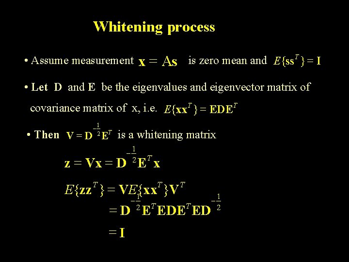
Whitening process • Assume measurement x = As is zero mean and E{ss. T } = I • Let D and E be the eigenvalues and eigenvector matrix of covariance matrix of x, i. e. E{xx. T } = EDET 1 2 • Then V = D ET is a whitening matrix 1 2 T = = z Vx D E x T T = E{zz } VE 1{xx }V 1 = D 2 ET ED 2 T =I

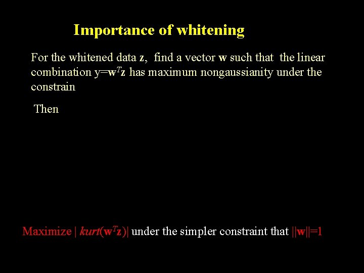
Importance of whitening For the whitened data z, find a vector w such that the linear combination y=w. Tz has maximum nongaussianity under the constrain Then Maximize | kurt(w. Tz)| under the simpler constraint that ||w||=1

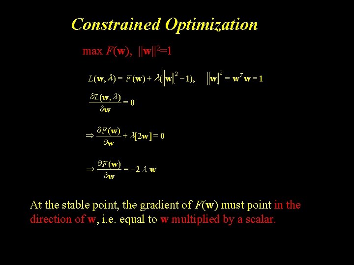
Constrained Optimization max F(w), ||w||2=1 2 L(w, l ) = F (w ) + l ( w 1), 2 w = w. T w = 1 ¶L(w , l ) =0 ¶w Þ ¶F (w ) + l[ 2 w ] = 0 ¶w Þ ¶F (w ) = 2 l w ¶w At the stable point, the gradient of F(w) must point in the direction of w, i. e. equal to w multiplied by a scalar.

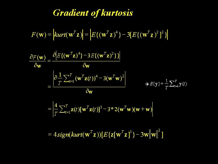
Gradient of kurtosis T T 4 T 2 2 F (w ) = kurt (w z ) = E{(w z ) } 3[ E{(w z ) ] } ¶F (w ) = ¶w ¶ E{(w T z ) 4 } 3 E{(w T z ) 2 }} ¶w ¶ = = 1 T T 4 T 2 ( w z ( t )) 3 ( w w ) å T t =1 ¶w Q E{y} = 4 T T 3 T z ( t )[ w z ( t )] 3 * 2 ( w w )(w + w ) å t =1 T 2 = 4 sign(kurt(w. T z))[E{z[w. T z]3 } 3 w w ] 1 T å y(t ) T t =1

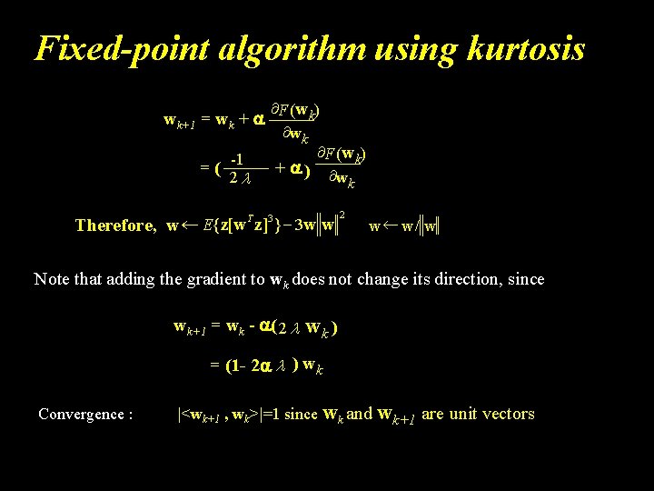
Fixed-point algorithm using kurtosis wk+1 = wk + =( -1 2 l ¶F (wk) ¶wk ¶F (wk) + ) ¶w k Therefore, w E{z[w T z ]3} 3 w w 2 w w/ w Note that adding the gradient to wk does not change its direction, since wk+1 = wk - ( 2 l wk ) = (1 - 2 l ) wk Convergence : |<wk+1 , wk>|=1 since wk and wk+1 are unit vectors

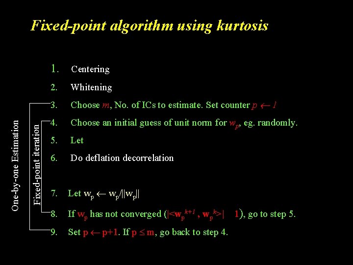
Fixed-point algorithm using kurtosis Fixed-point iteration One-by-one Estimation 1. Centering 2. Whitening 3. Choose m, No. of ICs to estimate. Set counter p 1 4. Choose an initial guess of unit norm for wp, eg. randomly. 5. Let 6. Do deflation decorrelation 7. Let wp wp/||wp|| 8. If wp has not converged (|<wpk+1 , wpk>| 9. Set p p+1. If p m, go back to step 4. 1), go to step 5.

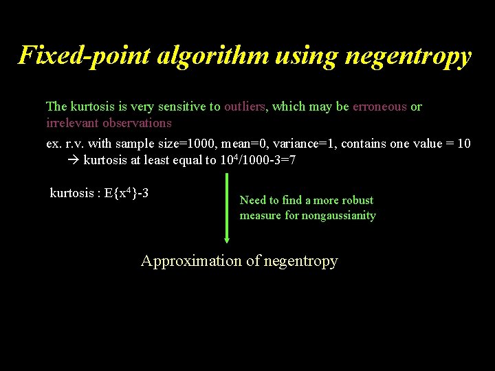
Fixed-point algorithm using negentropy The kurtosis is very sensitive to outliers, which may be erroneous or irrelevant observations ex. r. v. with sample size=1000, mean=0, variance=1, contains one value = 10 kurtosis at least equal to 104/1000 -3=7 kurtosis : E{x 4}-3 Need to find a more robust measure for nongaussianity Approximation of negentropy

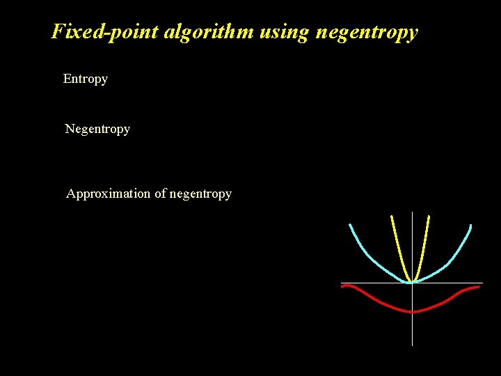
Fixed-point algorithm using negentropy Entropy Negentropy Approximation of negentropy

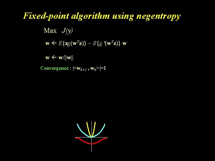
Fixed-point algorithm using negentropy Max J(y) w E{zg(w. Tz)} E{g '(w. Tz)} w w w/||w|| Convergence : |<wk+1 , wk>|=1

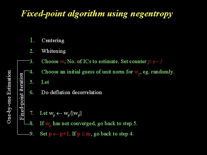
Fixed-point algorithm using negentropy Fixed-point iteration One-by-one Estimation 1. Centering 2. Whitening 3. Choose m, No. of ICs to estimate. Set counter p 1 4. Choose an initial guess of unit norm for wp, eg. randomly. 5. Let 6. Do deflation decorrelation 7. Let wp wp/||wp|| 8. If wp has not converged, go back to step 5. 9. Set p p+1. If p m, go back to step 4.

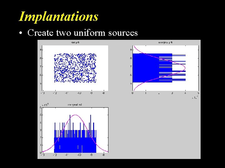
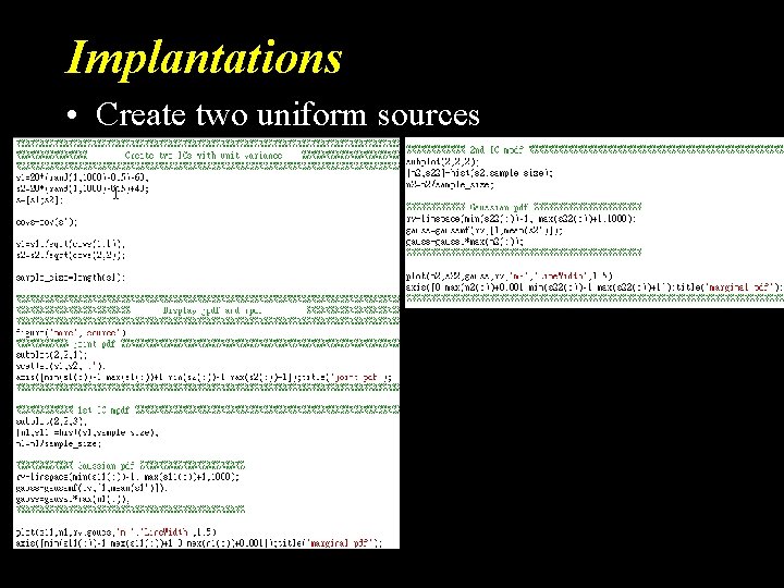
Implantations • Create two uniform sources

Implantations • Create two uniform sources

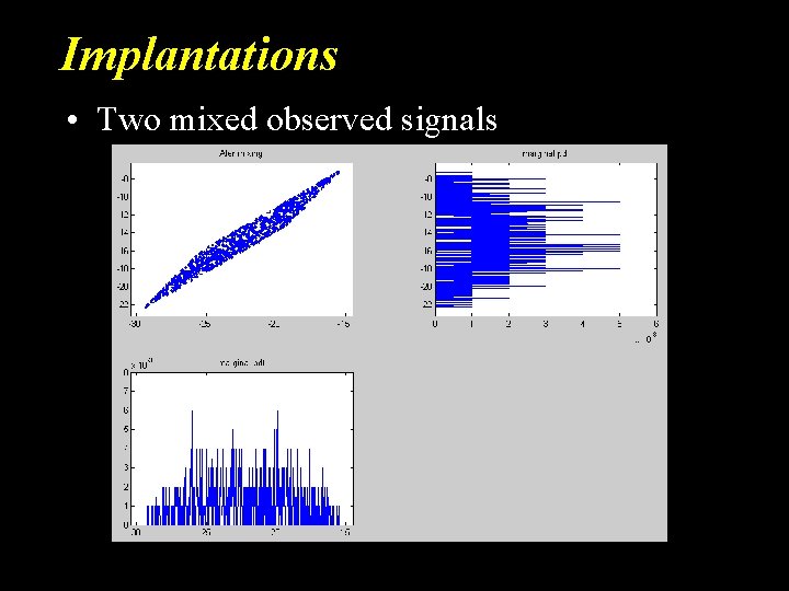
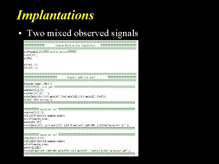
Implantations • Two mixed observed signals

Implantations • Two mixed observed signals

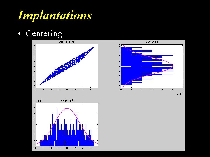
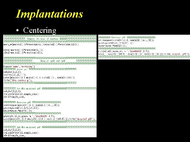
Implantations • Centering

Implantations • Centering

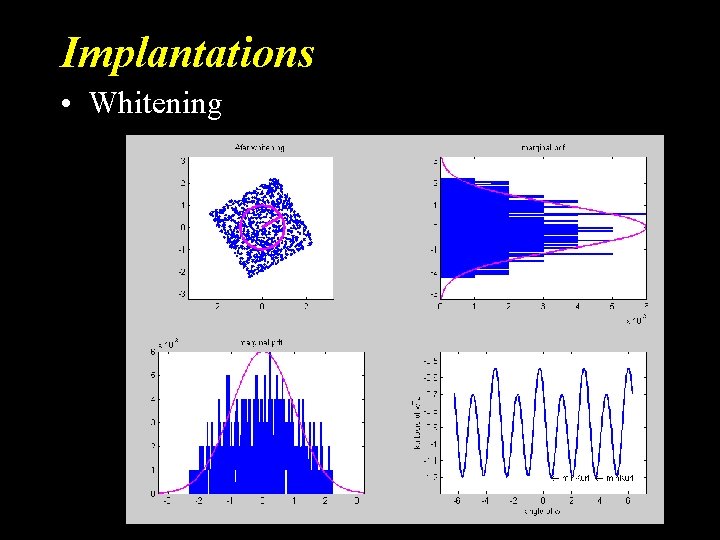
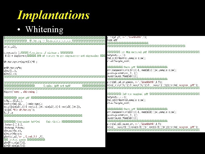
Implantations • Whitening

Implantations • Whitening

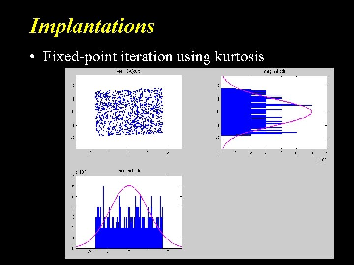
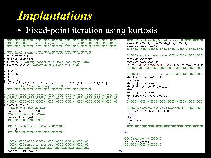
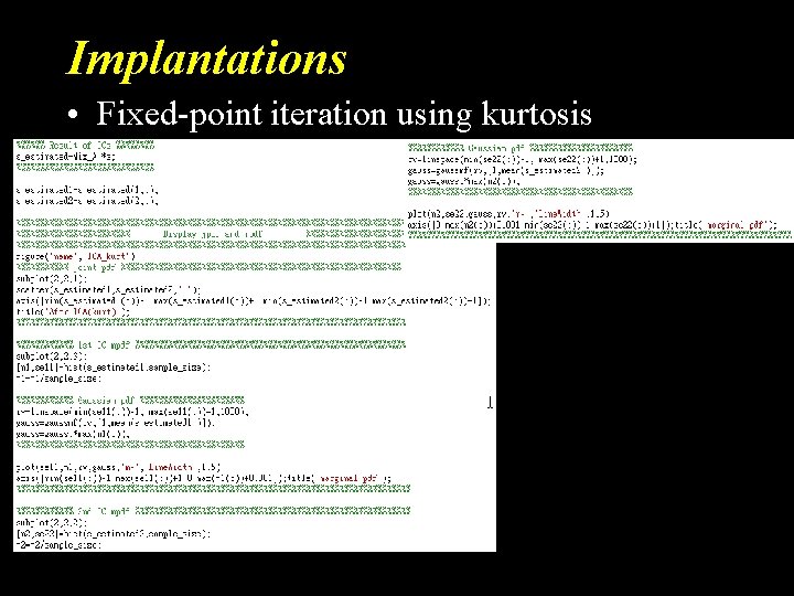
Implantations • Fixed-point iteration using kurtosis

Implantations • Fixed-point iteration using kurtosis

Implantations • Fixed-point iteration using kurtosis

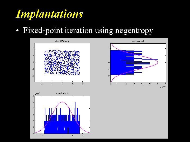
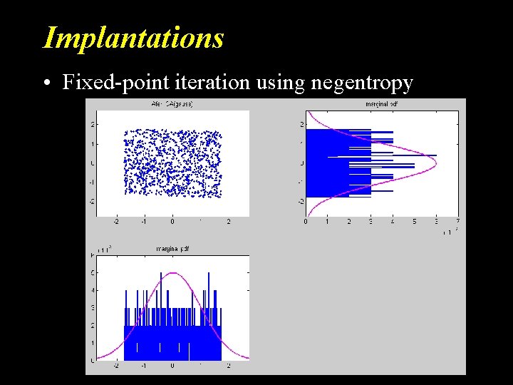
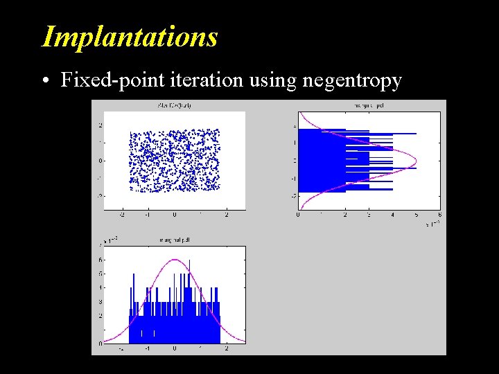
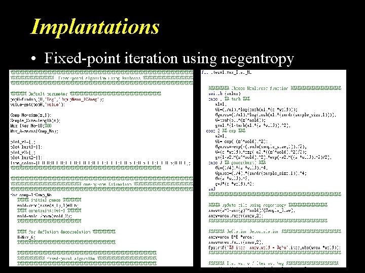
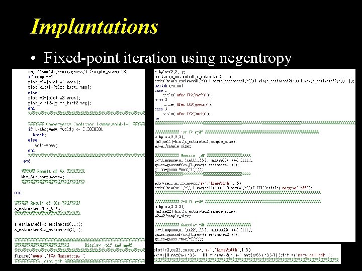
Implantations • Fixed-point iteration using negentropy

Implantations • Fixed-point iteration using negentropy

Implantations • Fixed-point iteration using negentropy

Implantations • Fixed-point iteration using negentropy

Implantations • Fixed-point iteration using negentropy

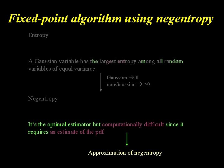
Fixed-point algorithm using negentropy Entropy A Gaussian variable has the largest entropy among all random variables of equal variance Gaussian 0 non. Gaussian >0 Negentropy It’s the optimal estimator but computationally difficult since it requires an estimate of the pdf Approximation of negentropy

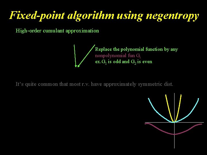
Fixed-point algorithm using negentropy High-order cumulant approximation Replace the polynomial function by any nonpolynomial fun Gi ex. G 1 is odd and G 2 is even It’s quite common that most r. v. have approximately symmetric dist.

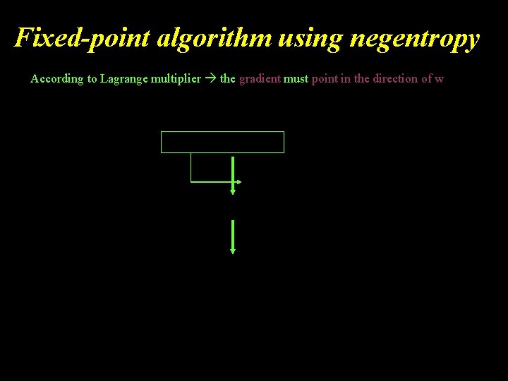
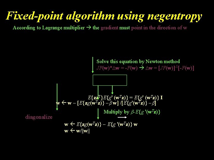
Fixed-point algorithm using negentropy According to Lagrange multiplier the gradient must point in the direction of w

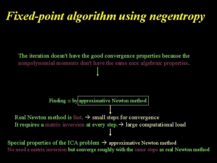
Fixed-point algorithm using negentropy The iteration doesn't have the good convergence properties because the nonpolynomial moments don't have the same nice algebraic properties. Finding by approximative Newton method Real Newton method is fast. small steps for convergence It requires a matrix inversion at every step. large computational load Special properties of the ICA problem approximative Newton method No need a matrix inversion but converge roughly with the same steps as real Newton method

Fixed-point algorithm using negentropy According to Lagrange multiplier the gradient must point in the direction of w Solve this equation by Newton method JF(w)* w = -F(w) w = [JF(w)]-1[-F(w)] E{zz. T}E{g' (w. Tz)} = E{g' (w. Tz)} I w w [E{zg(w. Tz)} w] /[E{g'(w. Tz)} ] diagonalize Multiply by -E{g '(w. Tz)} w E{zg(w. Tz)} E{g '(w. Tz)} w w w/||w||

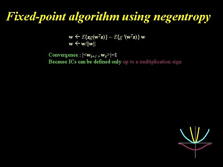
Fixed-point algorithm using negentropy w E{zg(w. Tz)} E{g '(w. Tz)} w w w/||w|| Convergence : |<wk+1 , wk>|=1 Because ICs can be defined only up to a multiplication sign