An Introduction to High Temperature QCD and Maximum

An Introduction to High Temperature QCD and Maximum Entropy Method Masayuki Asakawa Department of Physics, Osaka University Maximum Entropy Method Reviews: M. Jarrell and J. E. Gubernatis, Phys. Rept. 269 (1996) 133 T. Hatsuda, Y. Nakahara, and M. A. , Prog. Part. Nucl. Phys. 46 (2001) 459 hep-lat/0011040 July 2006 @National Tsing Hua University, Taiwan

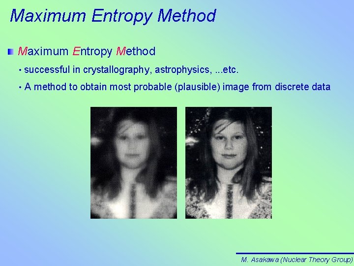
Maximum Entropy Method • successful in crystallography, astrophysics, . . . etc. • A method to obtain most probable (plausible) image from discrete data M. Asakawa (Nuclear Theory Group)

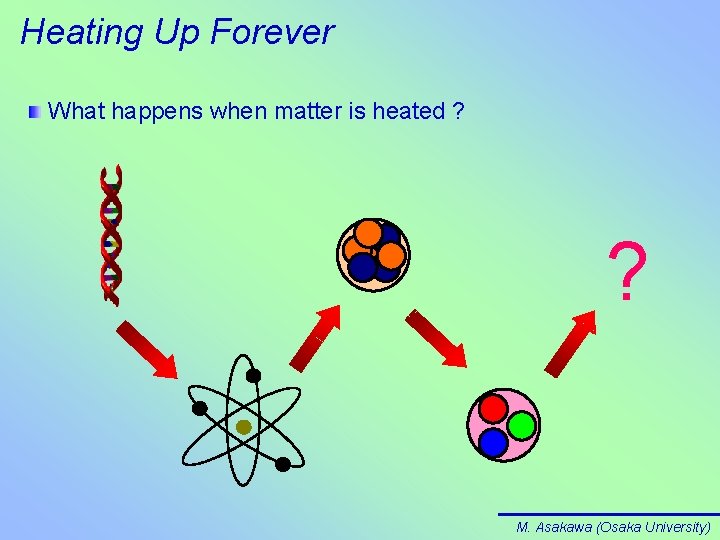
Heating Up Forever　 What happens when matter is heated ? 　 ? M. Asakawa (Osaka University)

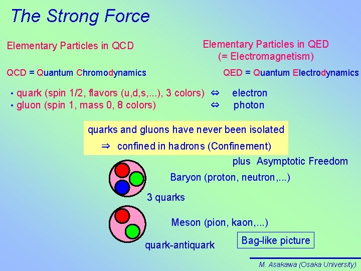
The Strong Force Elementary Particles in QED (= Electromagnetism) Elementary Particles in QCD = Quantum Chromodynamics QED = Quantum Electrodynamics • quark (spin 1/2, flavors (u, d, s, . . . ), 3 colors) ⇔　 electron • gluon (spin 1, mass 0, 8 colors)　　　　　　 ⇔ photon quarks and gluons have never been isolated ⇒　confined in hadrons (Confinement) plus Asymptotic Freedom Baryon (proton, neutron, . . . ) 3 quarks Meson (pion, kaon, . . . ) quark-antiquark Bag-like picture M. Asakawa (Osaka University)

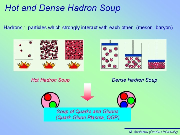
Hot and Dense Hadron Soup Hadrons : particles which strongly interact with each other　(meson, baryon) Hot Hadron Soup Dense Hadron Soup of Quarks and Gluons (Quark-Gluon Plasma, QGP) M. Asakawa (Osaka University)

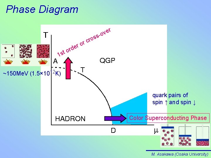
Phase Diagram r er d r st o o r cr s ve o s o 1 ~150 Me. V (1. 5× 1012 K) quark pairs of spin ↑ and spin ↓ Color Superconducting Phase M. Asakawa (Osaka University)

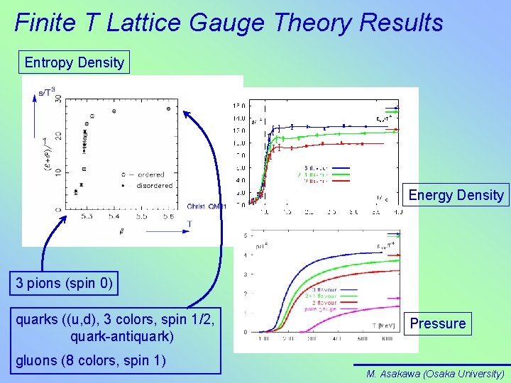
Finite T Lattice Gauge Theory Results Entropy Density Energy Density 3 pions (spin 0) quarks ((u, d), 3 colors, spin 1/2, quark-antiquark) Pressure gluons (8 colors, spin 1) M. Asakawa (Osaka University)

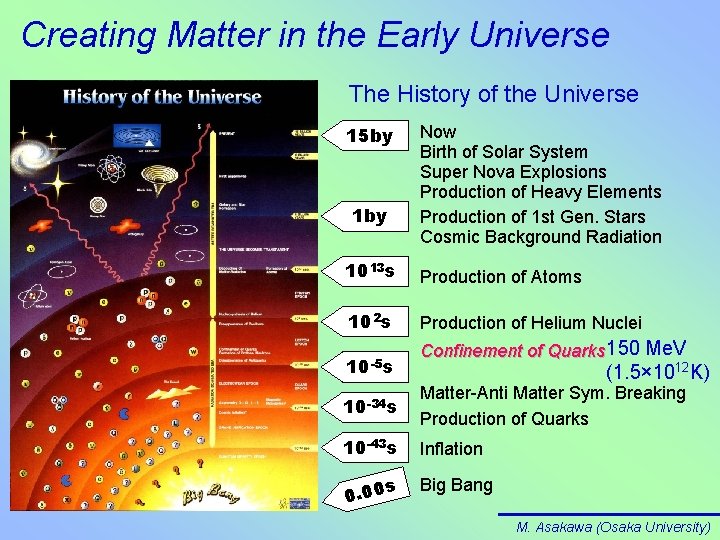
Creating Matter in the Early Universe The History of the Universe 15 by 1 by Now Birth of Solar System Super Nova Explosions Production of Heavy Elements Production of 1 st Gen. Stars Cosmic Background Radiation 1013 s Production of Atoms 102 s Production of Helium Nuclei 10 -5 s Confinement of Quarks 150 Me. V (1. 5× 1012 K) 10 -34 s Matter-Anti Matter Sym. Breaking Production of Quarks 10 -43 s Inflation s 0. 00 Big Bang M. Asakawa (Osaka University)

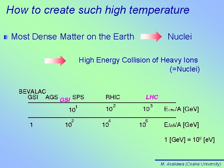
How to create such high temperature Most Dense Matter on the Earth　 Nuclei High Energy Collision of Heavy Ions (=Nuclei) 1 [Ge. V] = 109 [e. V] M. Asakawa (Osaka University)

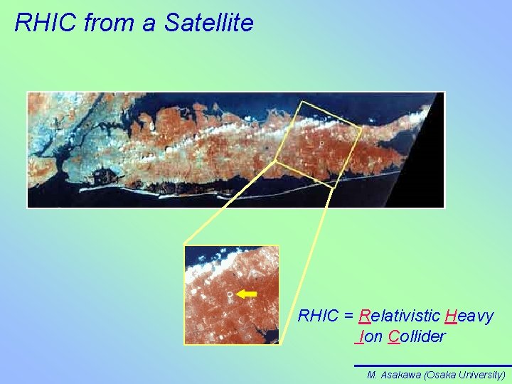
RHIC from a Satellite RHIC = Relativistic Heavy Ion Collider M. Asakawa (Osaka University)

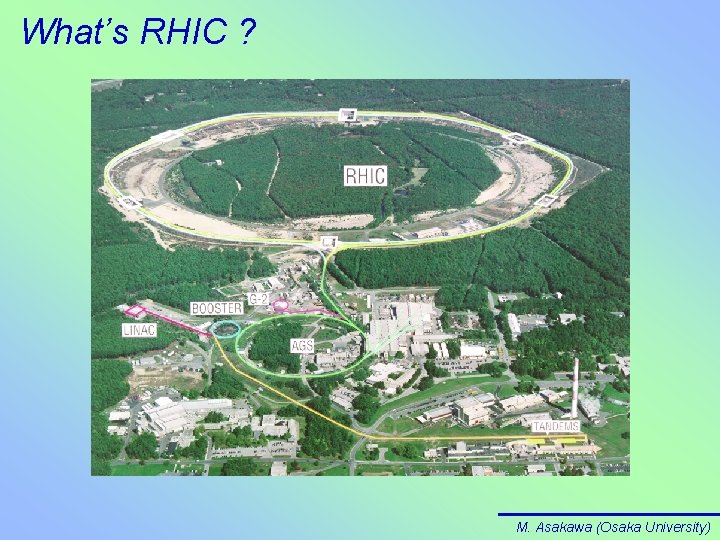
What’s RHIC ? M. Asakawa (Osaka University)

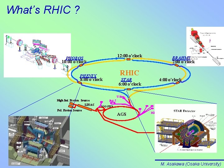
What’s RHIC ? 12: 00 o’clock PHOBOS 10: 00 o’clock RHIC PHENIX 8: 00 o’clock High Int. Proton Source LINAC Pol. Proton Source BRAHMS 2: 00 o’clock STAR 6: 00 o’clock m g-2 4: 00 o’clock U-line BOOSTER AGS HEP/NP TANDE MS M. Asakawa (Osaka University)

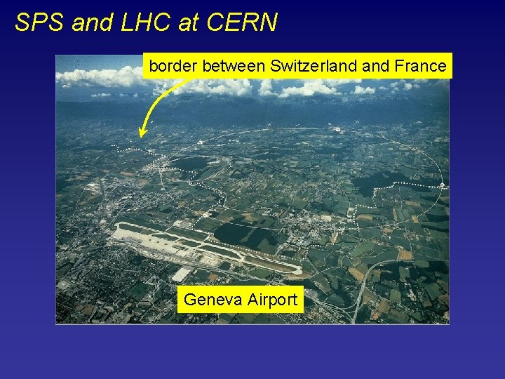
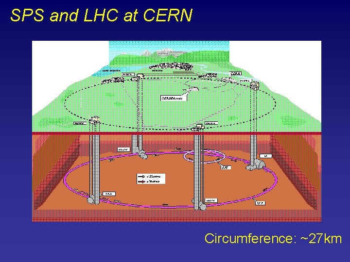
SPS and LHC at CERN border between Switzerland France Geneva Airport

SPS and LHC at CERN Circumference: ~27 km

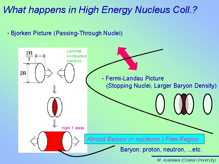
What happens in High Energy Nucleus Coll. ? • Bjorken Picture (Passing-Through Nuclei) • Fermi-Landau Picture (Stopping Nuclei, Larger Baryon Density) Almost Baryon (= nucleons ) Free Region Baryon: proton, neutron, . . . etc. M. Asakawa (Osaka University)

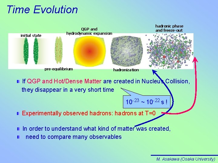
Time Evolution initial state hadronic phase and freeze-out QGP and hydrodynamic expansion pre-equilibrium hadronization If QGP and Hot/Dense Matter are created in Nucleus Collision, they disappear in a very short time 10 -23 ~ 10 -22 s ! Experimentally observed hadrons: hadrons at T=0 In order to understand what kind of matter was created, need to compare many observables M. Asakawa (Osaka University)

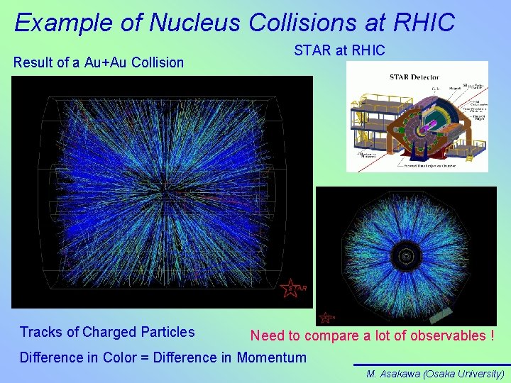
Example of Nucleus Collisions at RHIC Result of a Au+Au Collision Tracks of Charged Particles STAR at RHIC Need to compare a lot of observables ! Difference in Color = Difference in Momentum M. Asakawa (Osaka University)

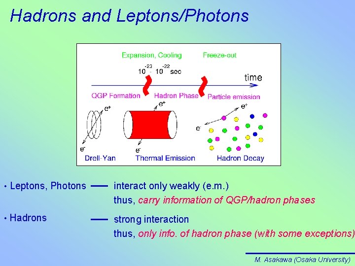
Hadrons and Leptons/Photons • Leptons, Photons interact only weakly (e. m. ) thus, carry information of QGP/hadron phases • Hadrons strong interaction thus, only info. of hadron phase (with some exceptions) M. Asakawa (Osaka University)

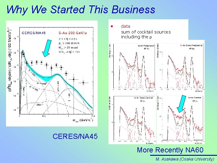
Why We Started This Business • data sum of cocktail sources including the CERES/NA 45 More Recently NA 60 M. Asakawa (Osaka University)

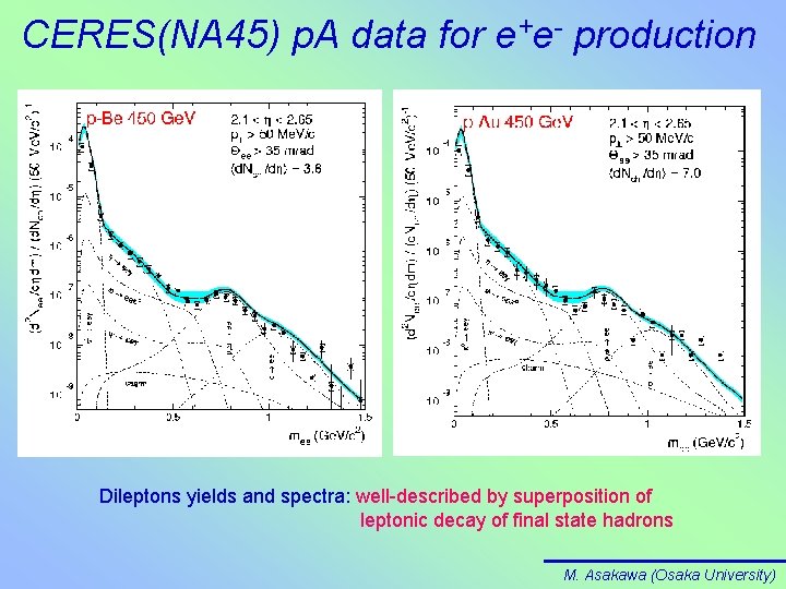
CERES(NA 45) p. A data for e+e- production Dileptons yields and spectra: well-described by superposition of leptonic decay of final state hadrons M. Asakawa (Osaka University)

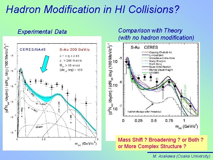
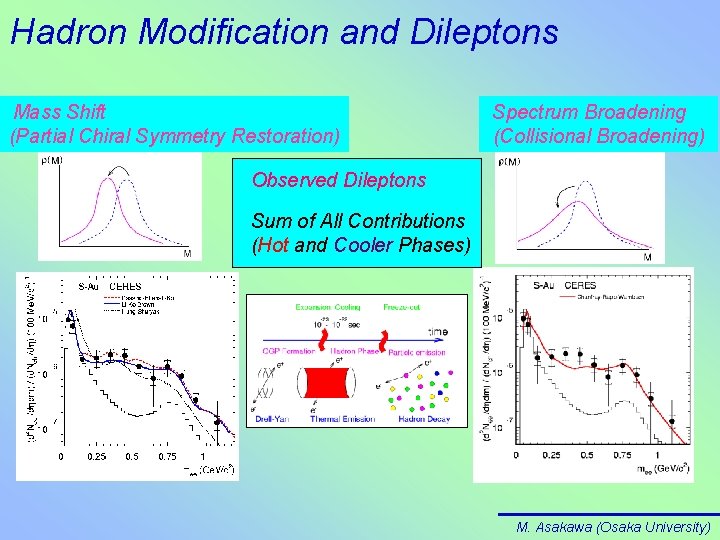
Hadron Modification in HI Collisions? Experimental Data Comparison with Theory (with no hadron modification) Mass Shift ? Broadening ? or Both ? or More Complex Structure ? M. Asakawa (Osaka University)

Why We Started This Business • data sum of cocktail sources including the CERES/NA 45 More Recently NA 60 M. Asakawa (Osaka University)

Hadron Modification and Dileptons Mass Shift (Partial Chiral Symmetry Restoration) Spectrum Broadening (Collisional Broadening) Observed Dileptons Sum of All Contributions (Hot and Cooler Phases) M. Asakawa (Osaka University)

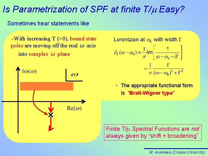
Is Parametrization of SPF at finite T/m Easy? Sometimes hear statements like –With increasing T (>0), bound state poles are moving off the real ω axis into complex ω plane ・ The appropriate functional form is “Breit-Wigner type” Finite T/ Spectral Functions are not always given by “shift + broadening” M. Asakawa (Osaka University)

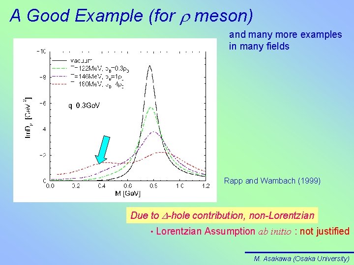
A Good Example (for r meson) and many more examples in many fields Rapp and Wambach (1999) Due to D-hole contribution, non-Lorentzian • Lorentzian Assumption ab initio : not justified M. Asakawa (Osaka University)

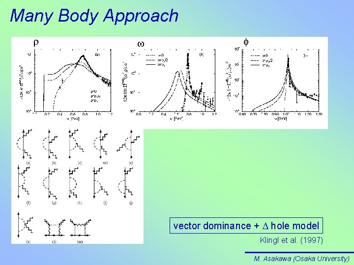
Many Body Approach vector dominance + D hole model Klingl et al. (1997) M. Asakawa (Osaka University)

A Good Example (for r meson) and many more examples in many fields Rapp and Wambach (1999) Due to D-hole contribution, non-Lorentzian • Lorentzian Assumption ab initio : not justified M. Asakawa (Osaka University)

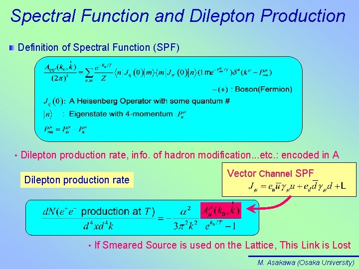
Spectral Function and Dilepton Production Definition of Spectral Function (SPF) • Dilepton production rate, info. of hadron modification. . . etc. : encoded in A Dilepton production rate • Vector Channel SPF If Smeared Source is used on the Lattice, This Link is Lost M. Asakawa (Osaka University)

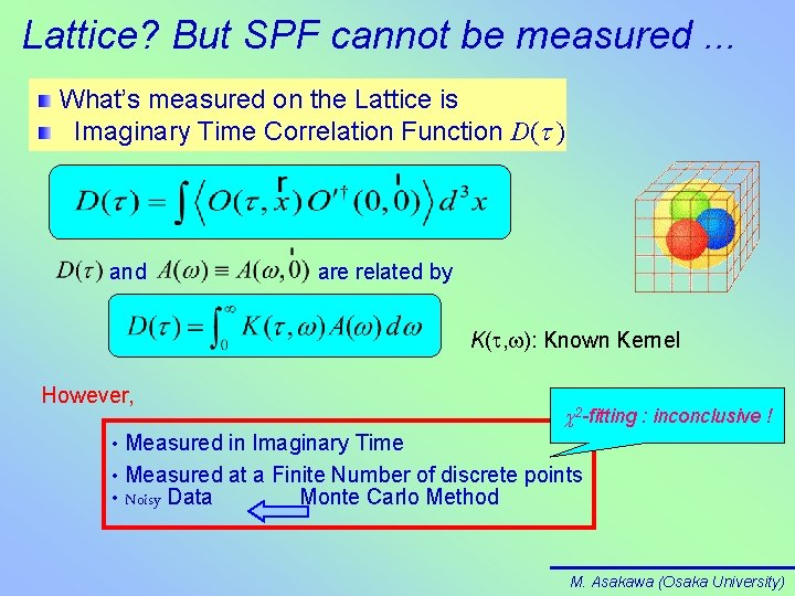
Lattice? But SPF cannot be measured. . . What’s measured on the Lattice is Imaginary Time Correlation Function D(t ) and are related by K(t, ): Known Kernel However, c 2 -fitting : inconclusive ! Measured in Imaginary Time • Measured at a Finite Number of discrete points • Noisy Data Monte Carlo Method • M. Asakawa (Osaka University)

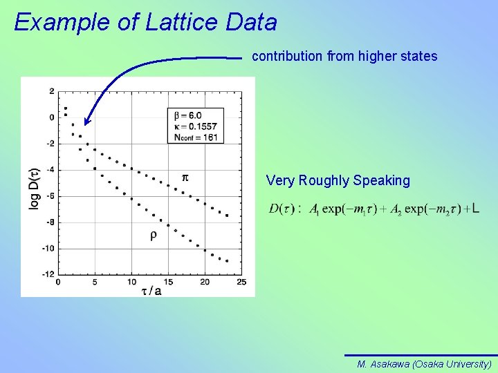
Example of Lattice Data contribution from higher states Very Roughly Speaking M. Asakawa (Osaka University)

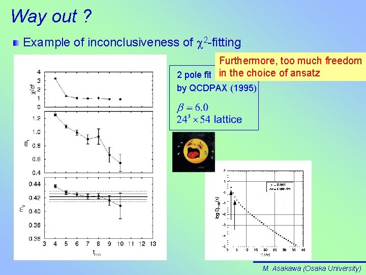
Way out ? Example of inconclusiveness of c 2 -fitting Furthermore, too much freedom 2 pole fit in the choice of ansatz by QCDPAX (1995) M. Asakawa (Osaka University)

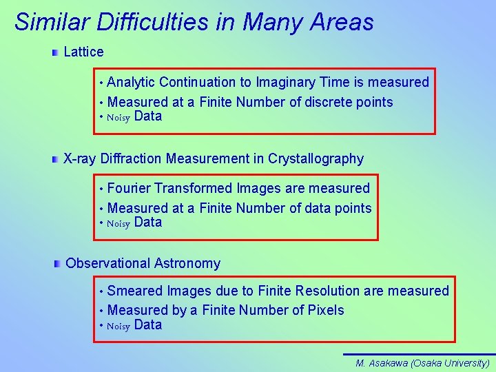
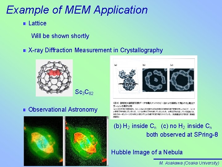
Similar Difficulties in Many Areas Lattice Analytic Continuation to Imaginary Time is measured • Measured at a Finite Number of discrete points • Noisy Data • X-ray Diffraction Measurement in Crystallography Fourier Transformed Images are measured • Measured at a Finite Number of data points • Noisy Data • Observational Astronomy Smeared Images due to Finite Resolution are measured • Measured by a Finite Number of Pixels • Noisy Data • M. Asakawa (Osaka University)

Maximum Entropy Method • successful in crystallography, astrophysics, . . . etc. • A method to obtain most probable (plausible) image from discrete data M. Asakawa (Nuclear Theory Group)

Example of MEM Application Lattice Will be shown shortly X-ray Diffraction Measurement in Crystallography Sc 3 C 82 Observational Astronomy (b) H 2 inside Cn (c) no H 2 inside Cn both observed at SPring-8 Hubble Image of a Nebula M. Asakawa (Osaka University)

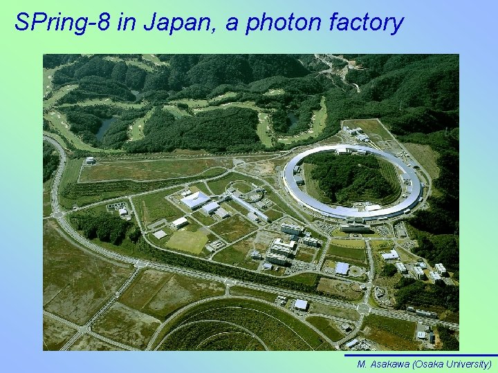
SPring-8 in Japan, a photon factory M. Asakawa (Osaka University)

Example of MEM Application Lattice Will be shown shortly X-ray Diffraction Measurement in Crystallography Sc 3 C 82 Observational Astronomy (b) H 2 inside Cn (c) no H 2 inside Cn both observed at SPring-8 Hubble Image of a Nebula M. Asakawa (Osaka University)

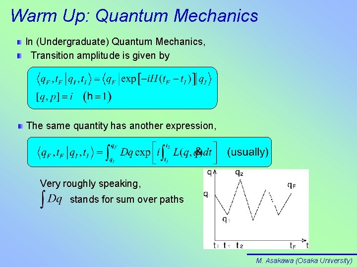
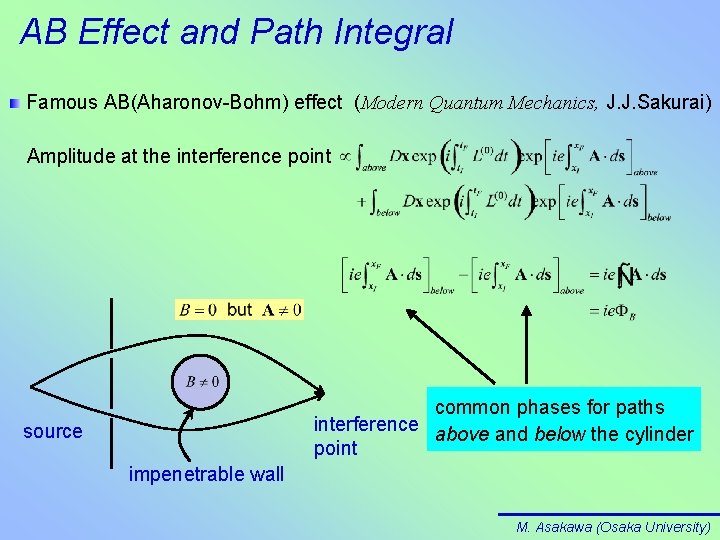
Warm Up: Quantum Mechanics In (Undergraduate) Quantum Mechanics, Transition amplitude is given by The same quantity has another expression, Very roughly speaking, stands for sum over paths M. Asakawa (Osaka University)

AB Effect and Path Integral Famous AB(Aharonov-Bohm) effect (Modern Quantum Mechanics, J. J. Sakurai) Amplitude at the interference point common phases for paths interference above and below the cylinder point source impenetrable wall M. Asakawa (Osaka University)

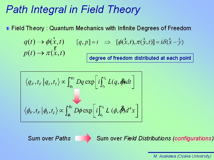
Path Integral in Field Theory : Quantum Mechanics with Infinite Degrees of Freedom degree of freedom distributed at each point Sum over Paths Sum over Field Distributions (configurations) M. Asakawa (Osaka University)

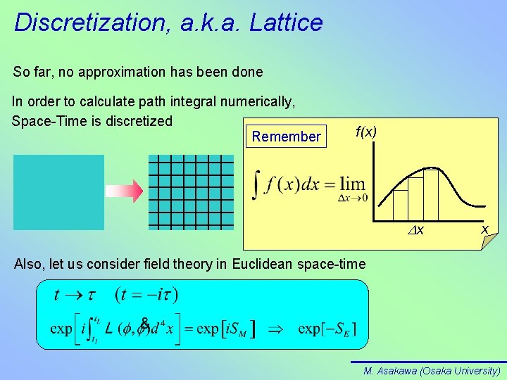
Discretization, a. k. a. Lattice So far, no approximation has been done In order to calculate path integral numerically, Space-Time is discretized Remember f(x) Dx x Also, let us consider field theory in Euclidean space-time M. Asakawa (Osaka University)

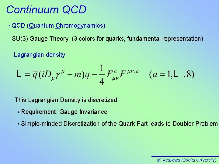
Continuum QCD • QCD (Quantum Chromodynamics) SU(3) Gauge Theory (3 colors for quarks, fundamental representation) Lagrangian density This Lagrangian Density is discretized • Requirement: Gauge Invariance • Simple-minded Discretization of the Quark Part leads to Doubler Problem M. Asakawa (Osaka University)

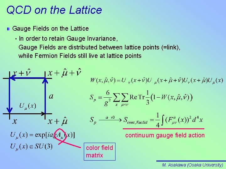
QCD on the Lattice Gauge Fields on the Lattice • In order to retain Gauge Invariance, Gauge Fields are distributed between lattice points (=link), while Fermion Fields still live at lattice points continuum gauge field action color field matrix M. Asakawa (Osaka University)

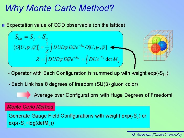
Why Monte Carlo Method? Expectation value of QCD observable (on the lattice) • Operator with Each Configuration is summed up with weight exp(-Slat) • Each Link has 8 degrees of freedom (SU(3) gluon color) Average over Configurations with Huge Degrees of Freedom! Monte Carlo Method Generate Gauge Field Configurations with weight exp(-Sp) or exp(-Sp+log(det. Mq)) M. Asakawa (Osaka University)

Lattice? But SPF cannot be measured. . . What’s measured on the Lattice is Imaginary Time Correlation Function D(t ) and are related by K(t, ): Known Kernel However, c 2 -fitting : inconclusive ! Measured in Imaginary Time • Measured at a Finite Number of discrete points • Noisy Data Monte Carlo Method • M. Asakawa (Osaka University)

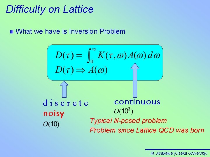
Difficulty on Lattice What we have is Inversion Problem discrete noisy continuous Typical ill-posed problem Problem since Lattice QCD was born M. Asakawa (Osaka University)

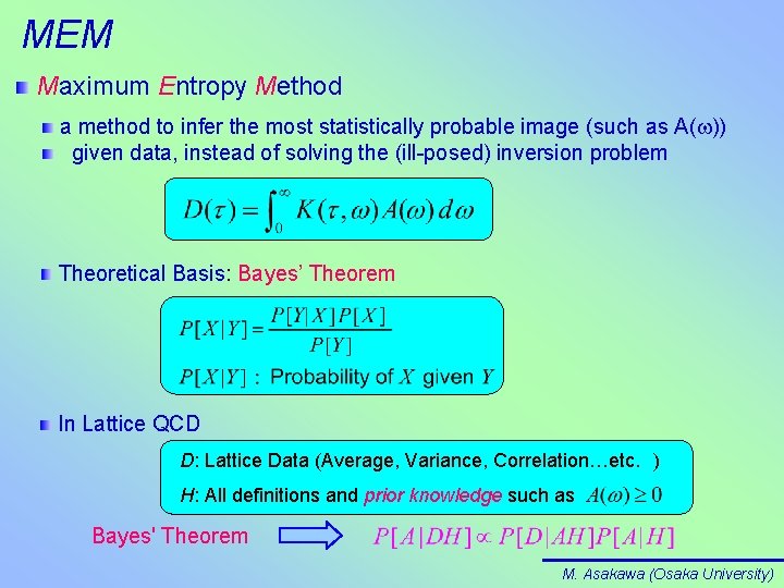
MEM Maximum Entropy Method a method to infer the most statistically probable image (such as A( )) given data, instead of solving the (ill-posed) inversion problem Theoretical Basis: Bayes’ Theorem In Lattice QCD D: Lattice Data (Average, Variance, Correlation…etc. 　) H: All definitions and prior knowledge such as Bayes' Theorem M. Asakawa (Osaka University)

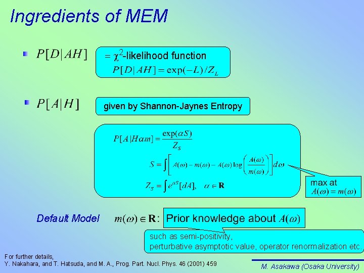
Ingredients of MEM = c 2 -likelihood function given by Shannon-Jaynes Entropy Default Model such as semi-positivity, perturbative asymptotic value, operator renormalization etc. For further details, Y. Nakahara, and T. Hatsuda, and M. A. , Prog. Part. Nucl. Phys. 46 (2001) 459 M. Asakawa (Osaka University)

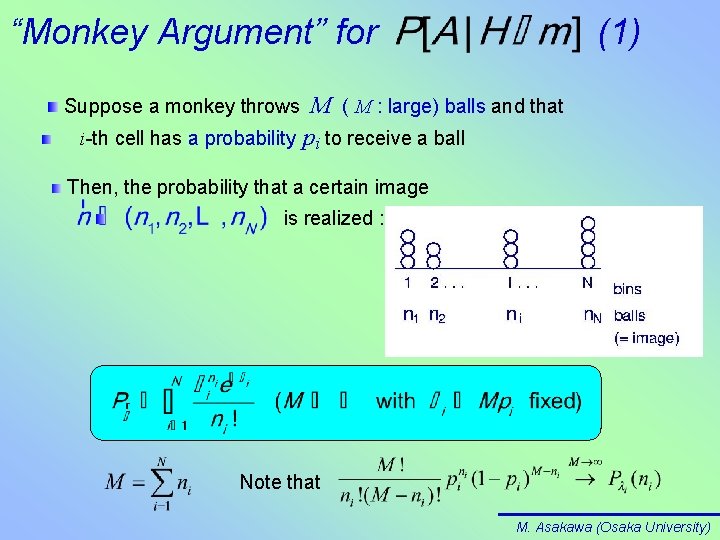
“Monkey Argument” for (1) M ( M : large) balls and that i-th cell has a probability pi to receive a ball Suppose a monkey throws Then, the probability that a certain image is realized : Note that M. Asakawa (Osaka University)

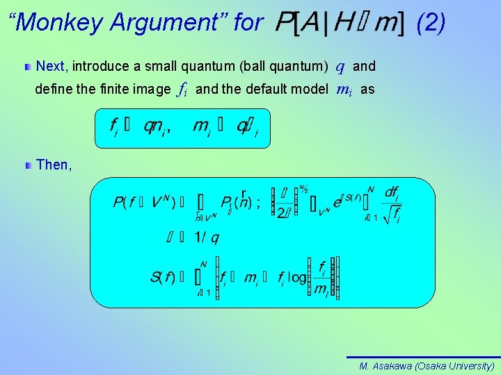
“Monkey Argument” for (2) q and define the finite image fi and the default model mi as Next, introduce a small quantum (ball quantum) Then, M. Asakawa (Osaka University)

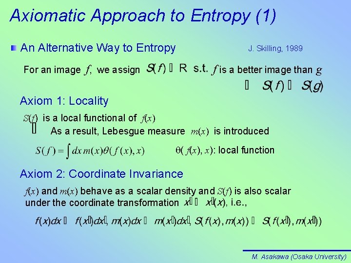
Axiomatic Approach to Entropy (1) An Alternative Way to Entropy For an image f, we assign J. Skilling, 1989 f is a better image than g Axiom 1: Locality S(f) is a local functional of f(x) As a result, Lebesgue measure m(x) is introduced q( f(x), x): local function Axiom 2: Coordinate Invariance f(x) and m(x) behave as a scalar density and S(f) is also scalar under the coordinate transformation M. Asakawa (Osaka University)

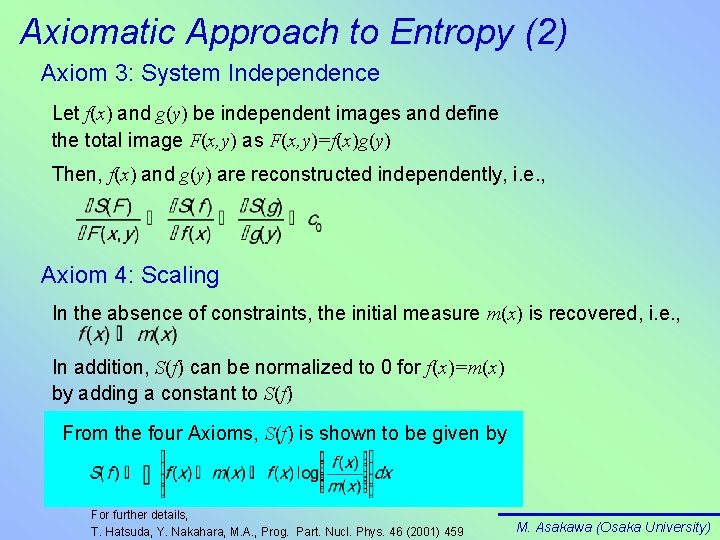
Axiomatic Approach to Entropy (2) Axiom 3: System Independence Let f(x) and g(y) be independent images and define the total image F(x, y) as F(x, y)=f(x)g(y) Then, f(x) and g(y) are reconstructed independently, i. e. , Axiom 4: Scaling In the absence of constraints, the initial measure m(x) is recovered, i. e. , In addition, S(f) can be normalized to 0 for f(x)=m(x) by adding a constant to S(f) From the four Axioms, S(f) is shown to be given by For further details, T. Hatsuda, Y. Nakahara, M. A. , Prog. Part. Nucl. Phys. 46 (2001) 459 M. Asakawa (Osaka University)

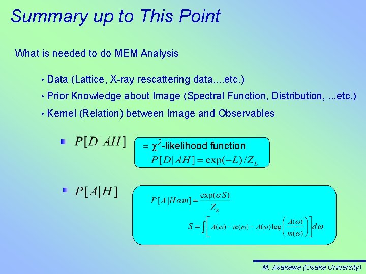
Summary up to This Point What is needed to do MEM Analysis • Data (Lattice, X-ray rescattering data, . . . etc. ) • Prior Knowledge about Image (Spectral Function, Distribution, . . . etc. ) • Kernel (Relation) between Image and Observables = c 2 -likelihood function M. Asakawa (Osaka University)

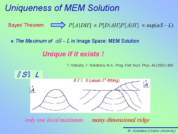
Uniqueness of MEM Solution Bayes' Theorem The Maximum of a. S - L in Image Space: MEM Solution Unique if it exists ! T. Hatsuda, Y. Nakahara, M. A. , Prog. Part. Nucl. Phys. 46 (2001) 459 only one local maximum many dimensional ridge M. Asakawa (Osaka University)

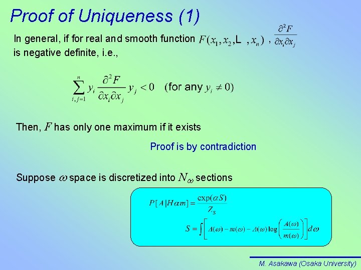
Proof of Uniqueness (1) In general, if for real and smooth function is negative definite, i. e. , , Then, F has only one maximum if it exists Proof is by contradiction Suppose w space is discretized into Nw sections M. Asakawa (Osaka University)

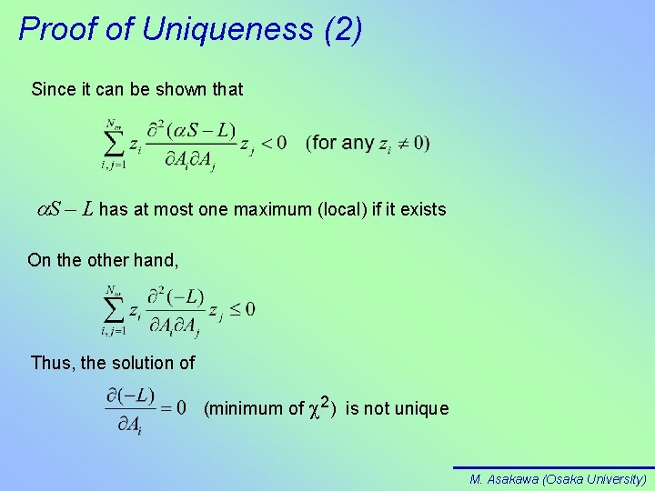
Proof of Uniqueness (2) Since it can be shown that a. S – L has at most one maximum (local) if it exists On the other hand, Thus, the solution of (minimum of c 2) is not unique M. Asakawa (Osaka University)

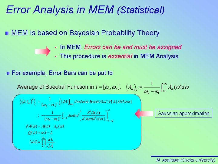
Error Analysis in MEM (Statistical) MEM is based on Bayesian Probability Theory • In MEM, Errors can be and must be assigned • This procedure is essential in MEM Analysis For example, Error Bars can be put to Gaussian approximation M. Asakawa (Osaka University)

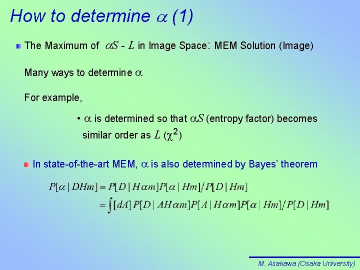
How to determine a (1) The Maximum of a. S - L in Image Space: MEM Solution (Image) Many ways to determine a For example, • a is determined so that a. S (entropy factor) becomes similar order as L (c 2) In state-of-the-art MEM, a is also determined by Bayes’ theorem M. Asakawa (Osaka University)

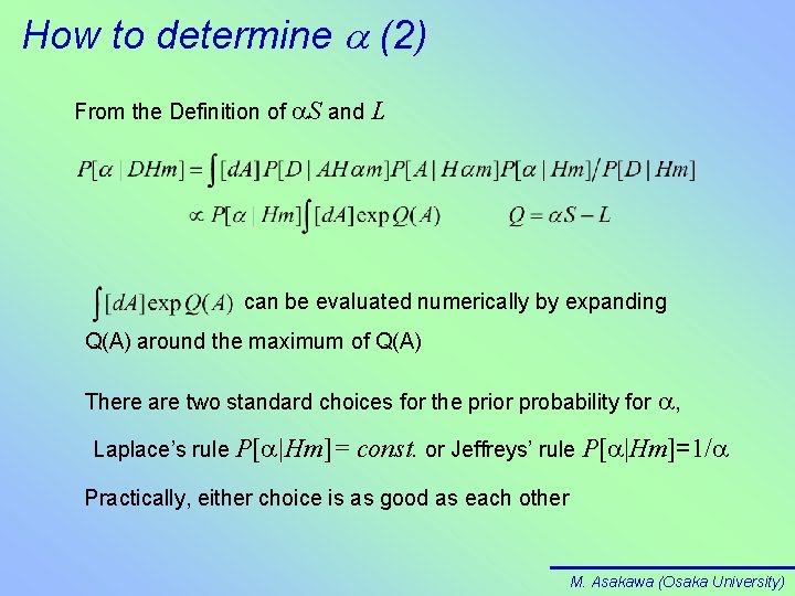
How to determine a (2) From the Definition of a. S and L can be evaluated numerically by expanding Q(A) around the maximum of Q(A) There are two standard choices for the prior probability for a, Laplace’s rule P[a|Hm]= const. or Jeffreys’ rule P[a|Hm]=1/a Practically, either choice is as good as each other M. Asakawa (Osaka University)

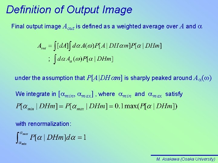
Definition of Output Image Final output image Aout is defined as a weighted average over A and a under the assumption that P[A|DHam] is sharply peaked around Aa( ) We integrate in [amin, amax] , where amin and amax satisfy with renormalization: M. Asakawa (Osaka University)

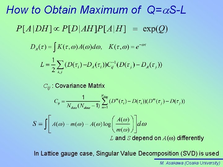
How to Obtain Maximum of Q=a. S-L Cij : Covariance Matrix L and S depend on A( ) differently In Lattice gauge case, Singular Value Decomposition (SVD) is used M. Asakawa (Osaka University)

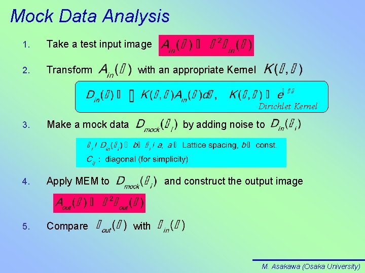
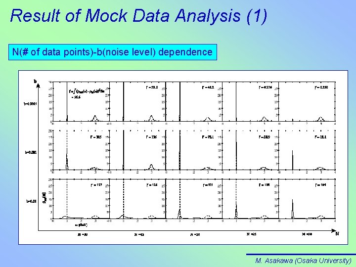
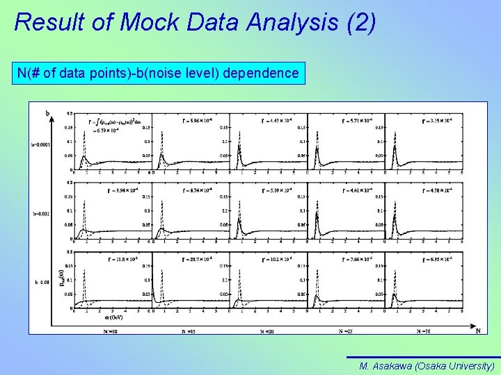
Mock Data Analysis 1. Take a test input image 2. Transform with an appropriate Kernel Dirichlet Kernel 3. Make a mock data 4. Apply MEM to 5. Compare by adding noise to 　 and construct the output image with M. Asakawa (Osaka University)

Result of Mock Data Analysis (1) N(# of data points)-b(noise level) dependence M. Asakawa (Osaka University)

Result of Mock Data Analysis (2) N(# of data points)-b(noise level) dependence M. Asakawa (Osaka University)

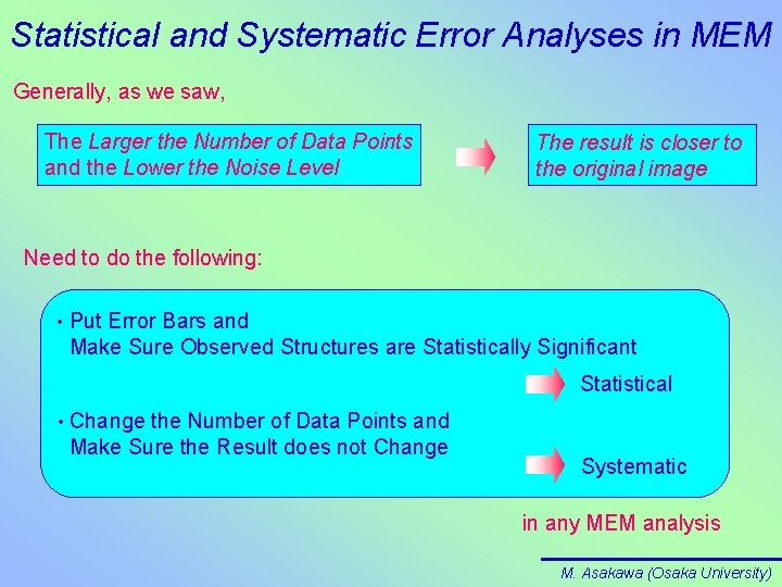
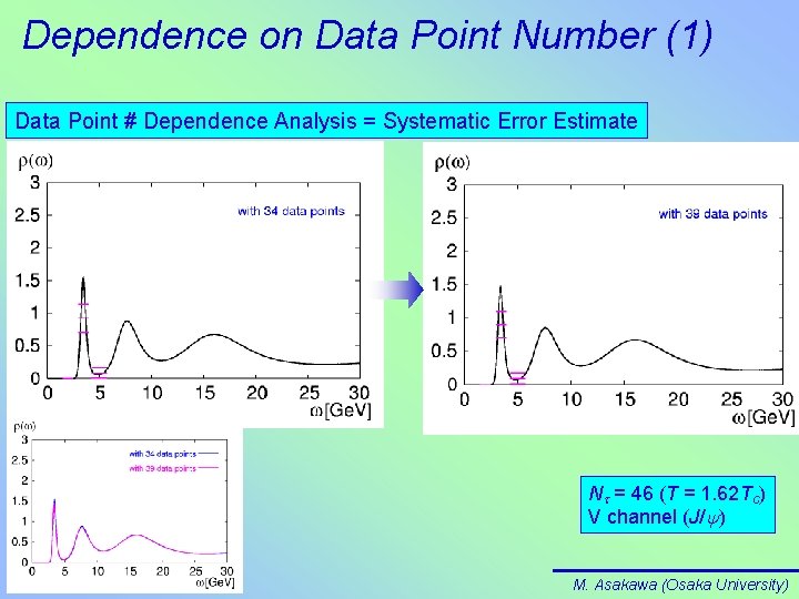
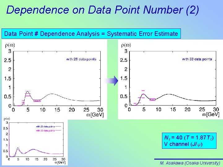
Statistical and Systematic Error Analyses in MEM Generally, as we saw, The Larger the Number of Data Points and the Lower the Noise Level The result is closer to the original image Need to do the following: • Put Error Bars and Make Sure Observed Structures are Statistically Significant Statistical • Change the Number of Data Points and Make Sure the Result does not Change Systematic in any MEM analysis M. Asakawa (Osaka University)

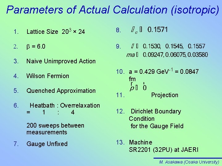
Parameters of Actual Calculation (isotropic) 1. Lattice Size 203 × 24 8. 2. b = 6. 0 9. 3. Naive Unimproved Action 4. Wilson Fermion 5. Quenched Approximation 6. Heatbath : Overrelaxation = 1 : 4 200 sweeps between measurements 7. Gauge Unfixed 10. a = 0. 429 Ge. V-1 = 0. 0847 fm 11. Projection 12. Dirichlet Boundary Condition for the Gauge Field 13. Machine SR 2201 (32 PU) at JAERI M. Asakawa (Osaka University)

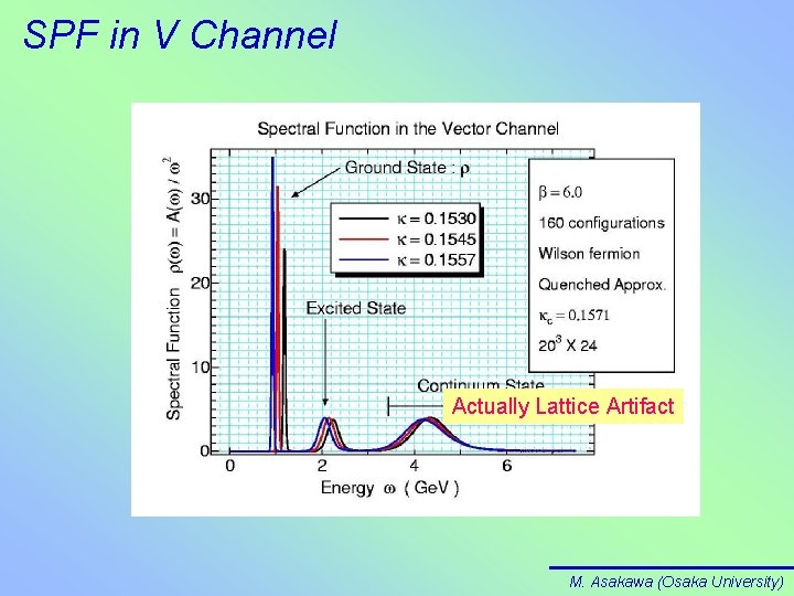
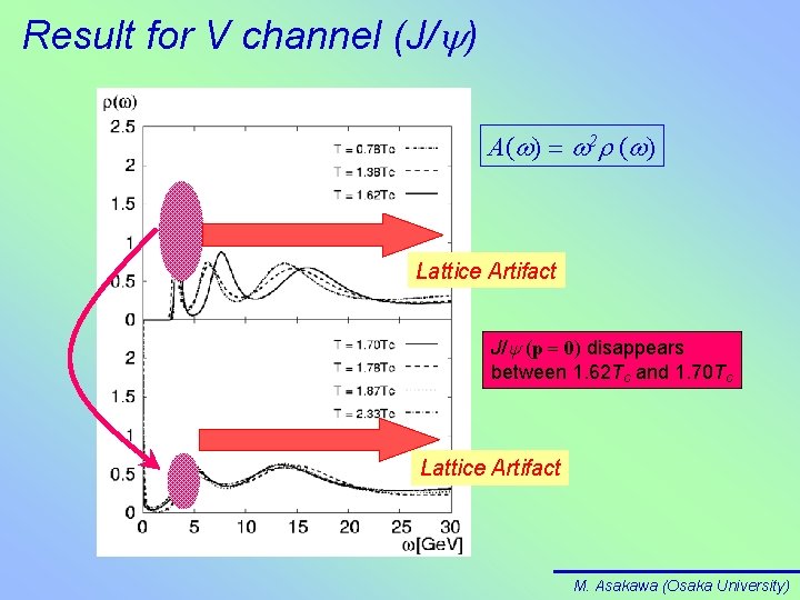
SPF in V Channel Actually Lattice Artifact M. Asakawa (Osaka University)

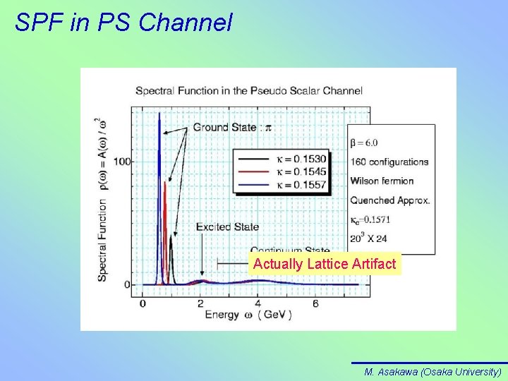
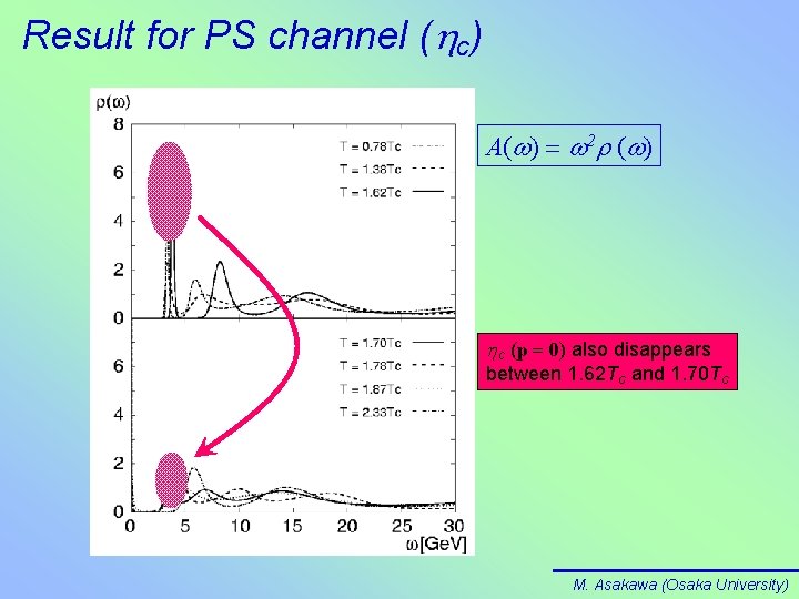
SPF in PS Channel Actually Lattice Artifact M. Asakawa (Osaka University)

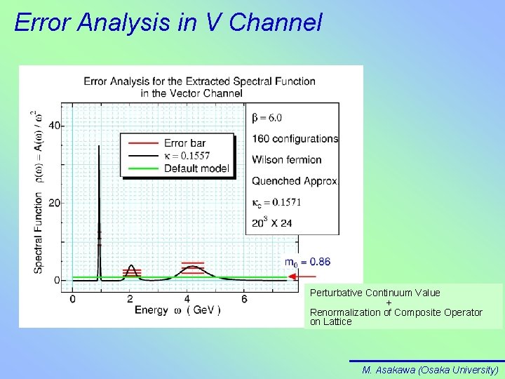
Error Analysis in V Channel Perturbative Continuum Value + Renormalization of Composite Operator on Lattice M. Asakawa (Osaka University)

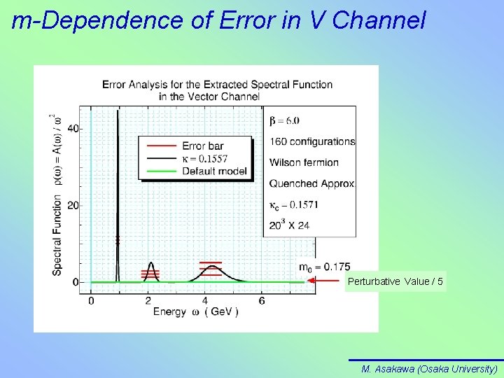
m-Dependence of Error in V Channel Perturbative Value / 5 M. Asakawa (Osaka University)

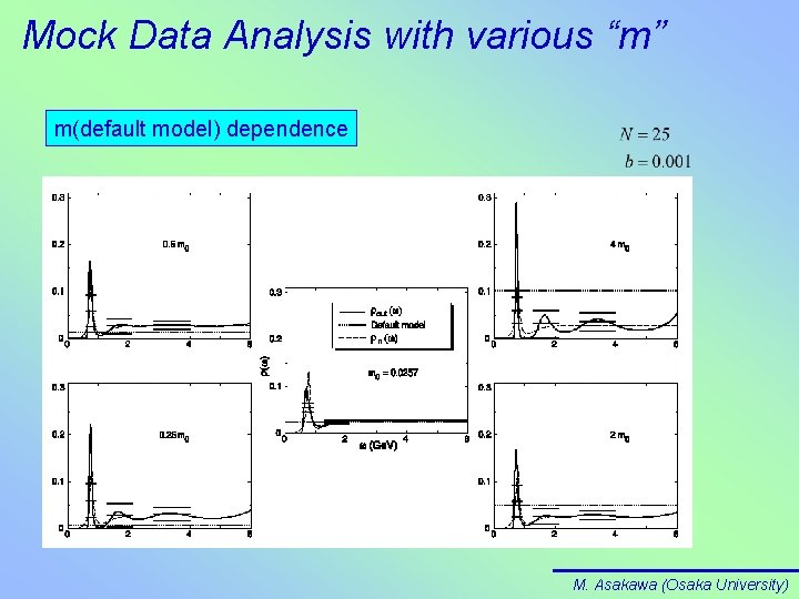
Mock Data Analysis with various “m” m(default model) dependence M. Asakawa (Osaka University)

How to determine m (default model)? So far, we have not discussed the m-dependence of results Mock Data analysis suggests the following: • Good Default Model tends to reproduce the input well Thus need to use prior knowledge (perturbative value, operator renormalization etc. ) as much as possible • Bad Default Model tends to produce fake structures (⇒Ringing) • However, if Bad Model is used, Error Bars also tend to increase • It looks like Fake Structures are within statistical error bars M. Asakawa (Osaka University)

N(# of Data Points) Dependence This must be carefully checked Need to do the following: • Put Error Bars and Make Sure Observed Structures are Statistically Significant Statistical • Change the Number of Data Points and Make Sure the Result does not Change Systematic in any MEM analysis This is important, in particular, in Finite T Lattice calculation, where # of Data points is often small M. Asakawa (Osaka University)

N dependence of Data (isotropic case) 403 * 30 lattice b = 6. 47, 150 confs. isotropic lattice (T<Tc) may depend on statistics, b, K, x, . . . etc. Nt, min @ 30 or larger M. Asakawa (Osaka University)

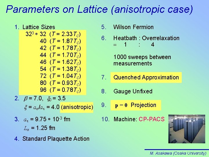
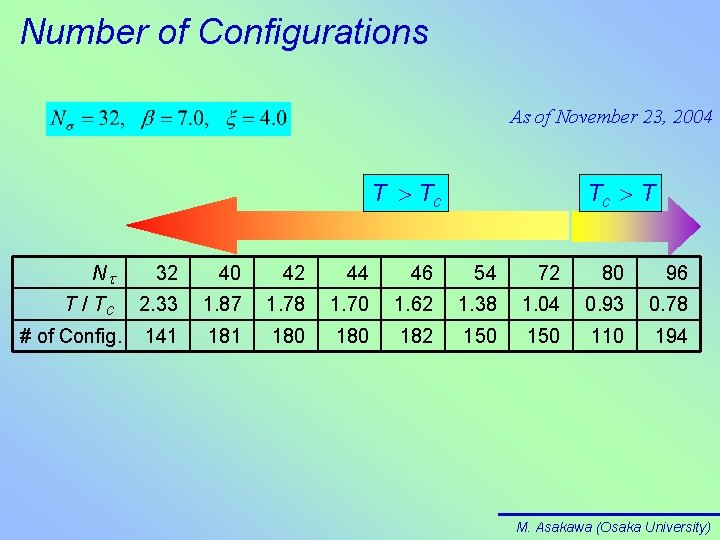
Parameters on Lattice (anisotropic case) 1. Lattice Sizes 323 * 32 (T = 2. 33 Tc) 40 (T = 1. 87 Tc) 42 (T = 1. 78 Tc) 44 (T = 1. 70 Tc) 46 (T = 1. 62 Tc) 54 (T = 1. 38 Tc) 72 (T = 1. 04 Tc) 80 (T = 0. 93 Tc) 96 (T = 0. 78 Tc) 2. b = 7. 0, x 0 = 3. 5 x = as/at = 4. 0 (anisotropic) 3. at = 9. 75 * 10 -3 fm Ls = 1. 25 fm 5. Wilson Fermion 6. Heatbath : Overrelaxation = 1 : 4 1000 sweeps between measurements 7. Quenched Approximation 8. Gauge Unfixed 9. p = 0 Projection 　　　 10. Machine: CP-PACS 4. Standard Plaquette Action M. Asakawa (Osaka University)

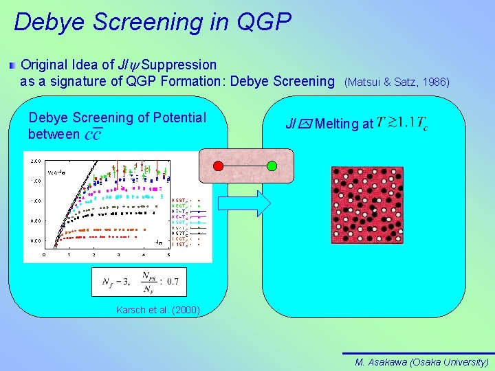
Debye Screening in QGP Original Idea of J/y Suppression as a signature of QGP Formation: Debye Screening of Potential between (Matsui & Satz, 1986) J/y Melting at Karsch et al. (2000) M. Asakawa (Osaka University)

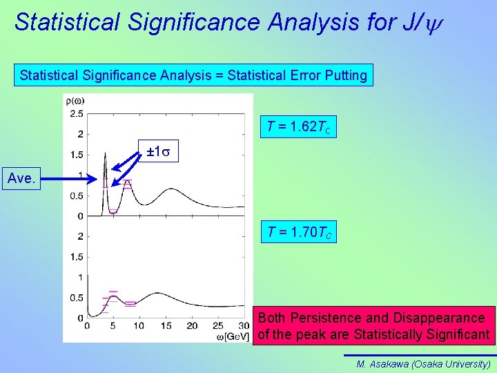
Result for V channel (J/y) A(w) = w 2 r (w) Lattice Artifact J/y (p = 0) disappears between 1. 62 Tc and 1. 70 Tc Lattice Artifact M. Asakawa (Osaka University)

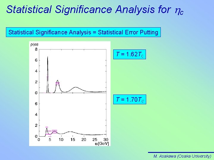
Result for PS channel (hc) A(w) = w 2 r (w) hc (p = 0) also disappears between 1. 62 Tc and 1. 70 Tc M. Asakawa (Osaka University)

Statistical Significance Analysis for J/y Statistical Significance Analysis = Statistical Error Putting T = 1. 62 Tc ± 1 s Ave. T = 1. 70 Tc Both Persistence and Disappearance of the peak are Statistically Significant M. Asakawa (Osaka University)

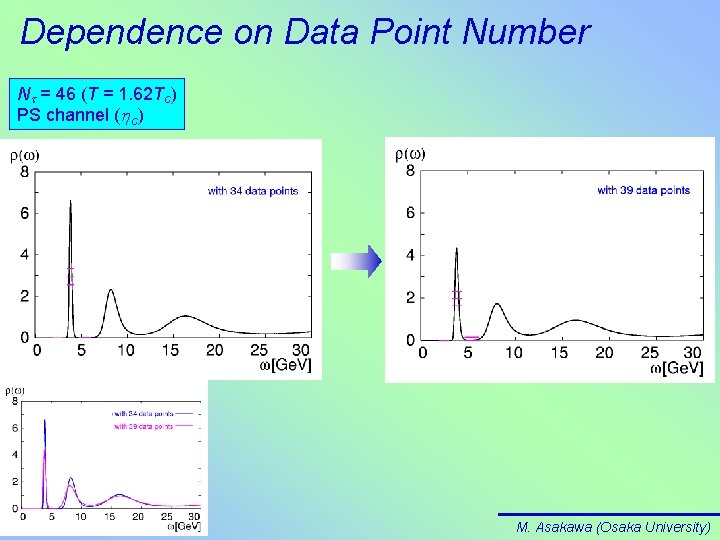
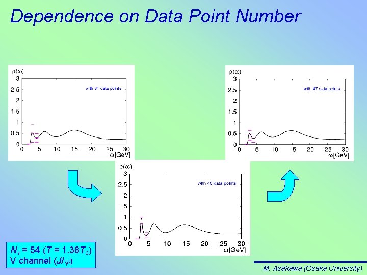
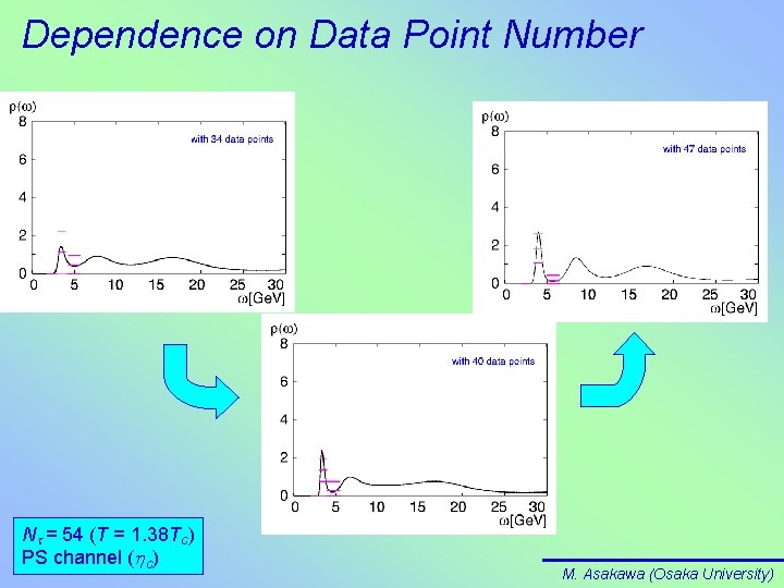
Dependence on Data Point Number (1) Data Point # Dependence Analysis = Systematic Error Estimate Nt = 46 (T = 1. 62 Tc) V channel (J/y) M. Asakawa (Osaka University)

Dependence on Data Point Number (2) Data Point # Dependence Analysis = Systematic Error Estimate Nt = 40 (T = 1. 87 Tc) V channel (J/y) M. Asakawa (Osaka University)

Back Up Slides M. Asakawa (Osaka University)

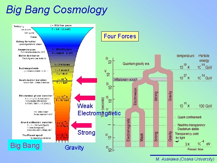
Big Bang Cosmology Four Forces Weak Electromagnetic Strong Big Bang Gravity M. Asakawa (Osaka University)

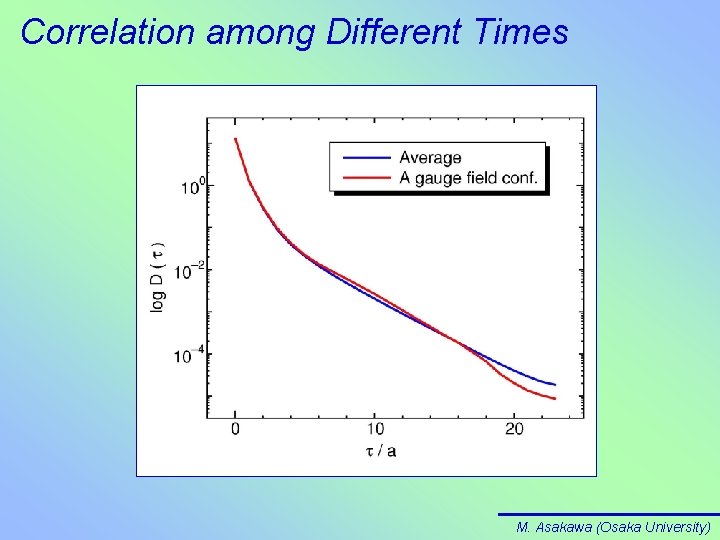
Correlation among Different Times M. Asakawa (Osaka University)

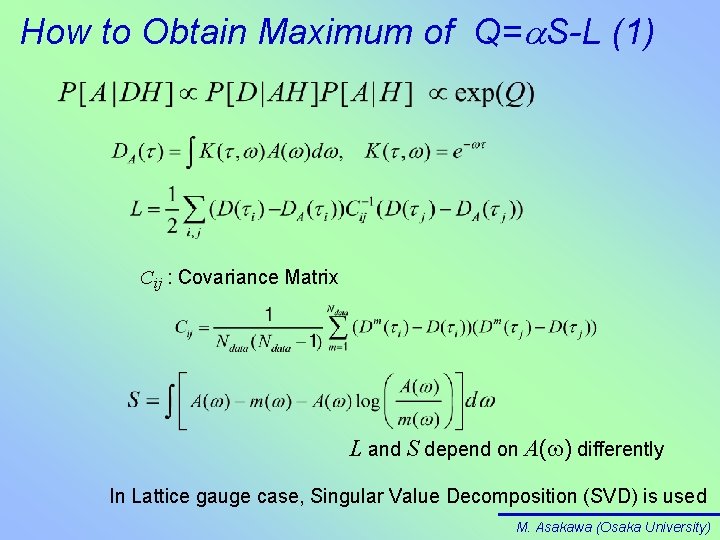
How to Obtain Maximum of Q=a. S-L (1) Cij : Covariance Matrix L and S depend on A( ) differently In Lattice gauge case, Singular Value Decomposition (SVD) is used M. Asakawa (Osaka University)

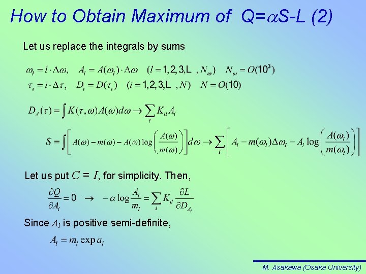
How to Obtain Maximum of Q=a. S-L (2) Let us replace the integrals by sums Let us put C = I, for simplicity. Then, Since Al is positive semi-definite, M. Asakawa (Osaka University)

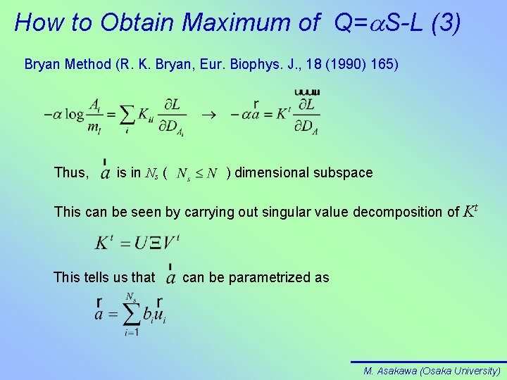
How to Obtain Maximum of Q=a. S-L (3) Bryan Method (R. K. Bryan, Eur. Biophys. J. , 18 (1990) 165) Thus, is in Ns ( ) dimensional subspace This can be seen by carrying out singular value decomposition of Kt This tells us that can be parametrized as M. Asakawa (Osaka University)

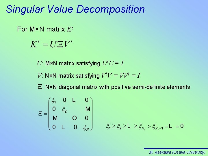
Singular Value Decomposition For M×N matrix Kt U: M×N matrix satisfying Ut. U = I V: N×N matrix satisfying Vt. V = VVt = I X: N×N diagonal matrix with positive semi-definite elements M. Asakawa (Osaka University)

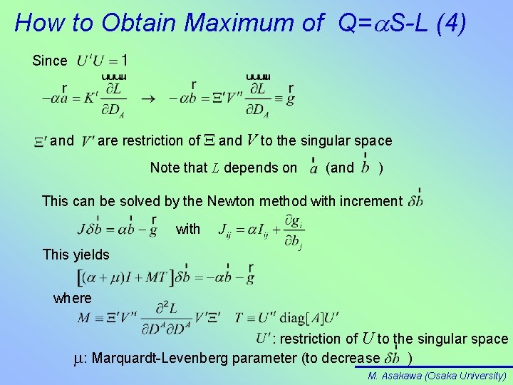
How to Obtain Maximum of Q=a. S-L (4) Since and are restriction of X and V to the singular space Note that L depends on (and ) This can be solved by the Newton method with increment with This yields where : restriction of U to the singular space : Marquardt-Levenberg parameter (to decrease ) M. Asakawa (Osaka University)

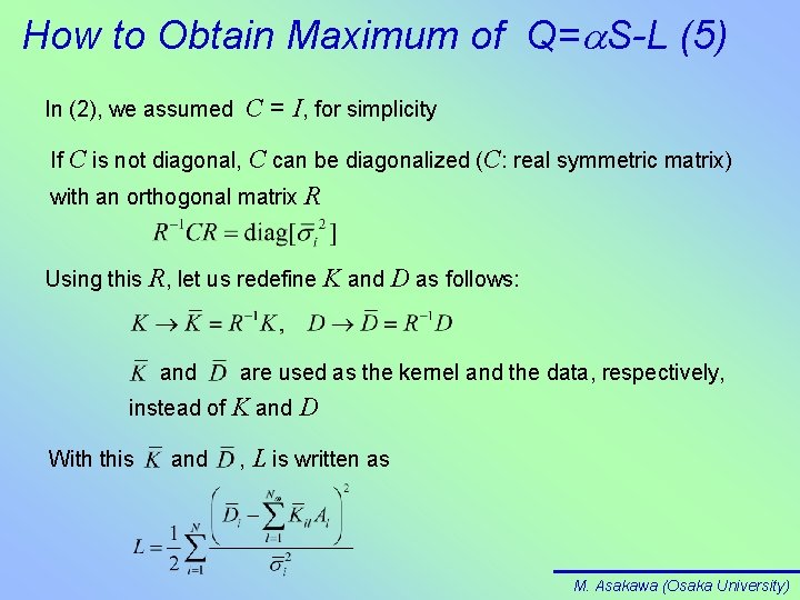
How to Obtain Maximum of Q=a. S-L (5) In (2), we assumed C = I, for simplicity If C is not diagonal, C can be diagonalized (C: real symmetric matrix) with an orthogonal matrix R Using this R, let us redefine K and D as follows: and are used as the kernel and the data, respectively, instead of K and D With this and , L is written as M. Asakawa (Osaka University)

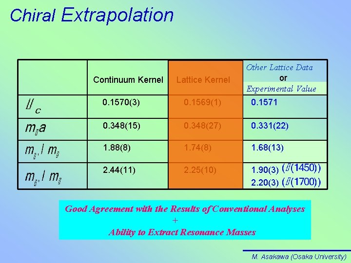
Chiral Extrapolation Continuum Kernel Lattice Kernel Other Lattice Data or Experimental Value 　　0. 1570(3) 0. 1569(1) 0. 1571 0. 348(15) 0. 348(27) 0. 331(22) 1. 88(8) 1. 74(8) 1. 68(13) 2. 44(11) 2. 25(10) 1. 90(3) 2. 20(3) Good Agreement with the Results of Conventional Analyses + Ability to Extract Resonance Masses M. Asakawa (Osaka University)

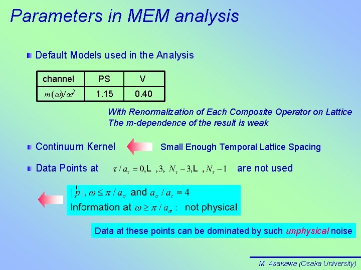
Parameters in MEM analysis Default Models used in the Analysis channel PS V m(w)/w 2 1. 15 0. 40 With Renormalization of Each Composite Operator on Lattice The m-dependence of the result is weak Continuum Kernel Data Points at Small Enough Temporal Lattice Spacing are not used 　　　　　　 Data at these points can be dominated by such unphysical noise M. Asakawa (Osaka University)

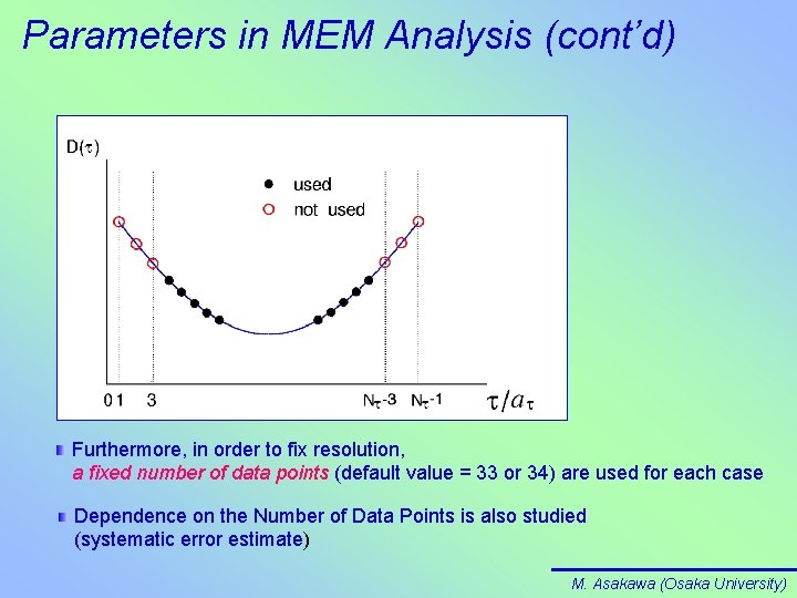
Parameters in MEM Analysis (cont’d) Furthermore, in order to fix resolution, a fixed number of data points (default value = 33 or 34) are used for each case Dependence on the Number of Data Points is also studied (systematic error estimate) M. Asakawa (Osaka University)

Number of Configurations As of November 23, 2004 T > Tc Tc > T Nt 32 40 42 44 46 54 72 80 96 T / Tc 2. 33 1. 87 1. 78 1. 70 1. 62 1. 38 1. 04 0. 93 0. 78 141 180 182 150 110 194 # of Config. M. Asakawa (Osaka University)

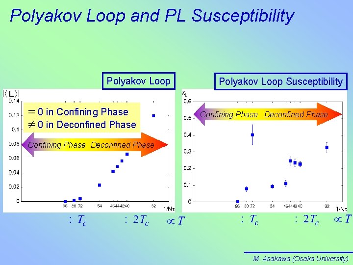
Polyakov Loop and PL Susceptibility Polyakov Loop 0 in Confining Phase 0 in Deconfined Phase Polyakov Loop Susceptibility Confining Phase Deconfined Phase M. Asakawa (Osaka University)

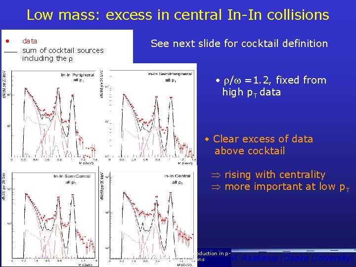
Low mass: excess in central In-In collisions • data sum of cocktail sources including the See next slide for cocktail definition • / =1. 2, fixed from high p. T data • Clear excess of data above cocktail rising with centrality more important at low p. T NA 60: dimuon and charm production in p. A and In-In collisions M. Asakawa (Osaka University)

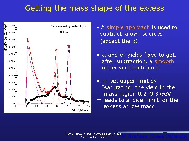
Getting the mass shape of the excess • A simple approach is used to subtract known sources (except the ) • and : yields fixed to get, after subtraction, a smooth underlying continuum • : set upper limit by “saturating” the yield in the mass region 0. 2– 0. 3 Ge. V leads to a lower limit for the excess at low mass NA 60: dimuon and charm production in p. A and In-In collisions M. Asakawa (Osaka University)

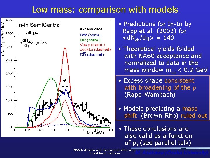
Low mass: comparison with models • Predictions for In-In by Rapp et al. (2003) for <d. Nch/d > = 140 • Theoretical yields folded with NA 60 acceptance and normalized to data in the mass window m < 0. 9 Ge. V • Excess shape consistent with broadening of the (Rapp-Wambach) • Models predicting a mass shift (Brown-Rho) ruled out • These conclusions are also valid as a function of p. T (see parallel talk) NA 60: dimuon and charm production in p. A and In-In collisions M. Asakawa (Osaka University)

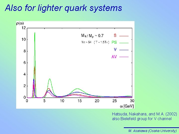
Also for lighter quark systems Hatsuda, Nakahara, and M. A. (2002) also Bielefeld group for V channel M. Asakawa (Osaka University)

Statistical Significance Analysis for hc Statistical Significance Analysis = Statistical Error Putting T = 1. 62 Tc T = 1. 70 Tc M. Asakawa (Osaka University)

Dependence on Data Point Number Nt = 46 (T = 1. 62 Tc) PS channel (hc) M. Asakawa (Osaka University)

Dependence on Data Point Number Nt = 54 (T = 1. 38 Tc) V channel (J/y) M. Asakawa (Osaka University)

Dependence on Data Point Number Nt = 54 (T = 1. 38 Tc) PS channel (hc) M. Asakawa (Osaka University)

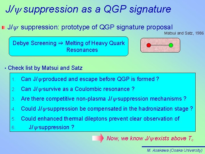
J/y suppression as a QGP signature J/y suppression: prototype of QGP signature proposal Matsui and Satz, 1986 Debye Screening ⇒ Melting of Heavy Quark Resonances • Check list by Matsui and Satz 1. Can J/y produced and escape before QGP is formed ? 2. Can J/y survive as a Coulombic resonance ? 3. Are there competitive non-plasma J/y suppression mechanisms ? 4. Could J/y suppression be compensated in the hadronization stage ? Could enhanced thermal dileptons prevent clear observation of 6. J/y suppression ? 5. Now, we know J/y exists above Tc M. Asakawa (Osaka University)

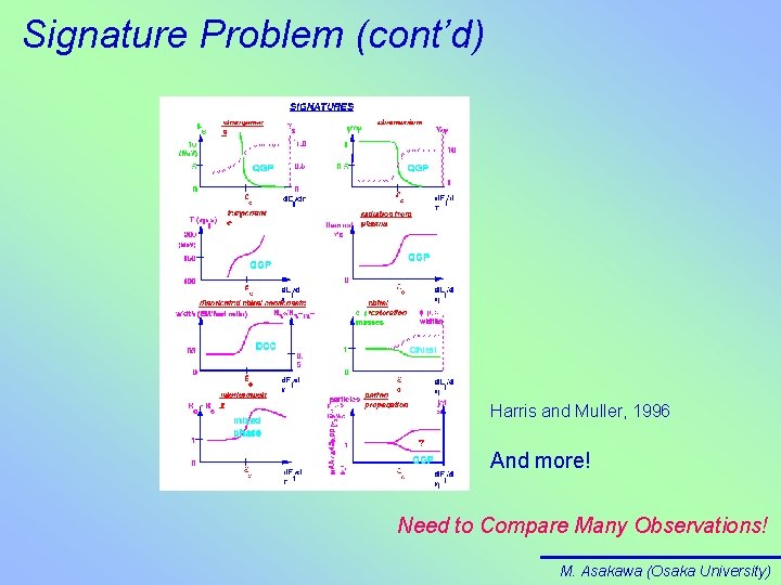
Signature Problem (cont’d) 　 Harris and Muller, 1996 And more! Need to Compare Many Observations! M. Asakawa (Osaka University)

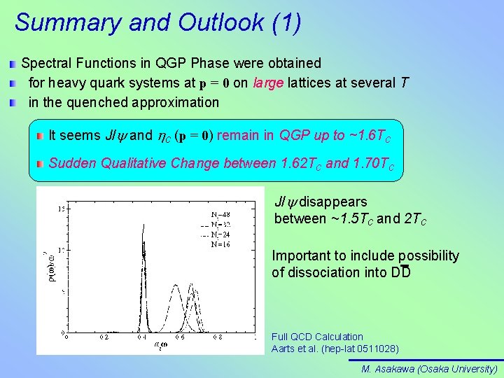
Summary and Outlook (1) Spectral Functions in QGP Phase were obtained for heavy quark systems at p = 0 on large lattices at several T in the quenched approximation It seems J/y and hc (p = 0) remain in QGP up to ~1. 6 Tc Sudden Qualitative Change between 1. 62 Tc and 1. 70 Tc • J/y disappears This result is, roughly, in accordance with between ~1. 5 Tc and 2 Tc other lattice calculations (e. g. , Bielefeld-BNL) and potential model analyses (e. g. , to C. Y. Wong) Important include possibility • dissociation into DD No finite p calculation forof J/y yet (Two Spectral Functions, Transverse and Longitudinal, for J/y at finite p ): ←　p. T dependence of J/y Suppression • QCD Calculation Non-Quench Calculation Full Started (Swansea-Dublin) Aarts et al. (hep-lat 0511028) M. Asakawa (Osaka University)

Summary and Outlook (2) Both Statistical and Systematic Error Estimates have been carefully carried out This must be carried out in any MEM analysis ~34 Data Points look sufficient to carry out MEM analysis on the present Lattice and with the current Statistics (But this is Lattice and Statistics dependent) Both Continuum and Thermodynamical (V→ ) Limits: Still Needed M. Asakawa (Osaka University)