An Introduction to Bioinformatics Comparing biological sequences 3

An Introduction to Bioinformatics Comparing biological sequences (3): Database searching and Multiple alignment

An Introduction to Bioinformatics Database searching • Goal: find similar (homologous) sequences of a query sequence in a sequence of database • Input: query sequence & database • Output: hits (pairwise alignments)

An Introduction to Bioinformatics Database searching • • Core: pair-wise alignment algorithm Speed (fast sequence comparison) Relevance of the search results (statistical tests) Recovering all information of interest • • The results depend of the search parameters like gap penalty, scoring matrix. Sometimes searches with more than one matrix should be preformed

An Introduction to Bioinformatics What program to use for searching? 1) BLAST is fastest and easily accessed on the Web • • limited sets of databases nice translation tools (BLASTX, TBLASTN) 2) FASTA • • • precise choice of databases more sensitive for DNA-DNA comparisons FASTX and TFASTX can find similarities in sequences with frameshifts 3) Smith-Waterman is slower, but more sensitive • • known as a “rigorous” or “exhaustive” search SSEARCH in GCG and standalone FASTA

An Introduction to Bioinformatics FASTA 1) Derived from logic of the dot plot • compute best diagonals from all frames of alignment 2) Word method looks for exact matches between words in query and test sequence • • hash tables (fast computer technique) DNA words are usually 6 bases protein words are 1 or 2 amino acids only searches for diagonals in region of word matches = faster searching

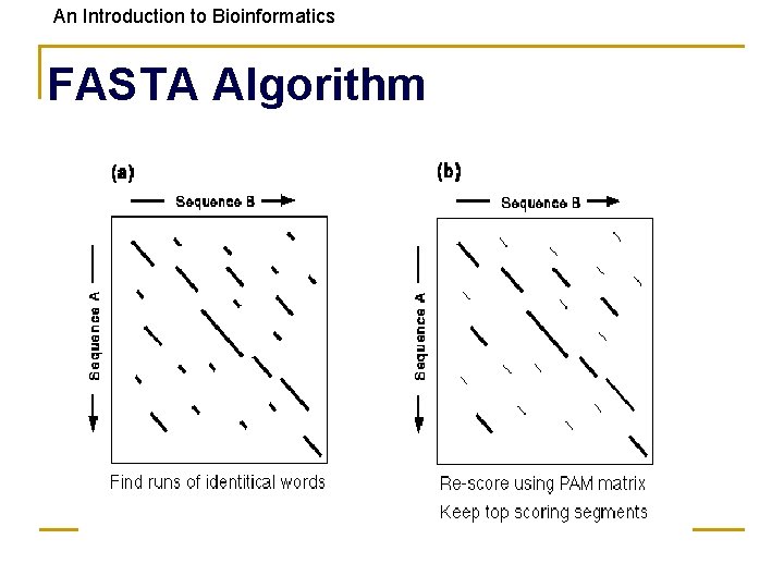
An Introduction to Bioinformatics FASTA Algorithm

An Introduction to Bioinformatics Makes Longest Diagonal 3) after all diagonals found, tries to join diagonals by adding gaps 4) computes alignments in regions of best diagonals

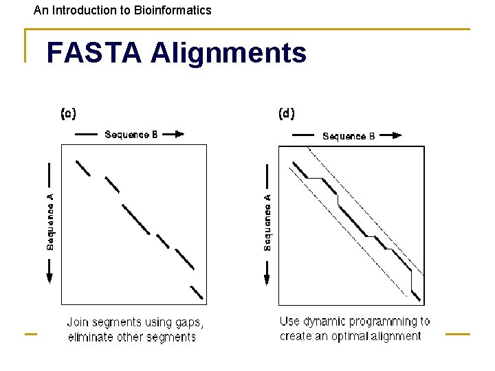
An Introduction to Bioinformatics FASTA Alignments

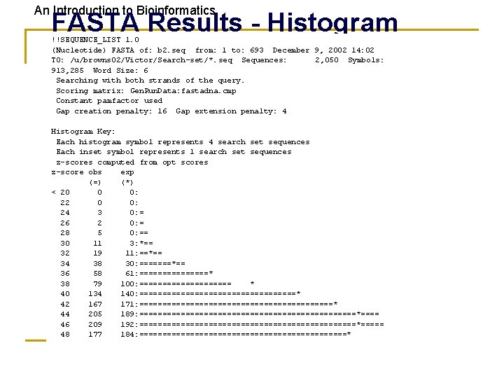
An Introduction to Bioinformatics FASTA Results - Histogram !!SEQUENCE_LIST 1. 0 (Nucleotide) FASTA of: b 2. seq from: 1 to: 693 December 9, 2002 14: 02 TO: /u/browns 02/Victor/Search-set/*. seq Sequences: 2, 050 Symbols: 913, 285 Word Size: 6 Searching with both strands of the query. Scoring matrix: Gen. Run. Data: fastadna. cmp Constant pamfactor used Gap creation penalty: 16 Gap extension penalty: 4 Histogram Key: Each histogram symbol represents 4 search set sequences Each inset symbol represents 1 search set sequences z-scores computed from opt scores z-score obs exp (=) (*) < 20 0 0: 22 0 0: 24 3 0: = 26 2 0: = 28 5 0: == 30 11 3: *== 32 19 11: ==*== 34 38 30: =======*== 36 58 61: ========* 38 79 100: ========== * 40 134 140: =================* 42 167 171: =====================* 44 205 189: ========================*==== 46 209 192: ========================*===== 48 177 184: =======================*

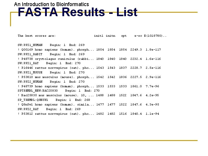
An Introduction to Bioinformatics FASTA Results - List The best scores are: init 1 initn SW: PPI 1_HUMAN Begin: 1 End: 269 ! Q 00169 homo sapiens (human). phosph. . . 1854 SW: PPI 1_RABIT Begin: 1 End: 269 ! P 48738 oryctolagus cuniculus (rabbi. . . 1840 SW: PPI 1_RAT Begin: 1 End: 270 ! P 16446 rattus norvegicus (rat). pho. . . 1543 SW: PPI 1_MOUSE Begin: 1 End: 270 ! P 53810 musculus (mouse). phosph. . . 1542 SW: PPI 2_HUMAN Begin: 1 End: 270 ! P 48739 homo sapiens (human). phosph. . . 1533 SPTREMBL_NEW: BAC 25830 Begin: 1 End: 270 ! Bac 25830 musculus (mouse). 10, . . . 1488 SP_TREMBL: Q 8 N 5 W 1 Begin: 1 End: 268 ! Q 8 n 5 w 1 homo sapiens (human). simila. . . 1477 SW: PPI 2_RAT Begin: 1 End: 269 ! P 53812 rattus norvegicus (rat). pho. . . 1482 opt z-sc E(1018780). . 1854 2249. 3 1. 8 e-117 1840 2232. 4 1. 6 e-116 1543 1837 2228. 7 2. 5 e-116 1542 1836 2227. 5 2. 9 e-116 1533 1861. 0 7. 7 e-96 1488 1522 1847. 6 4. 2 e-95 1477 1522 1847. 6 4. 3 e-95 1482 1516 1840. 4 1. 1 e-94

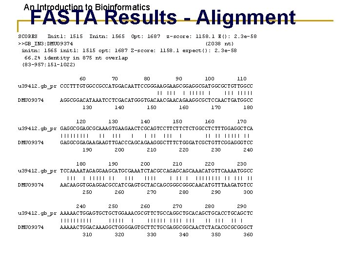
An Introduction to Bioinformatics FASTA Results - Alignment SCORES Init 1: 1515 Initn: 1565 Opt: 1687 z-score: 1158. 1 E(): 2. 3 e-58 >>GB_IN 3: DMU 09374 (2038 nt) initn: 1565 init 1: 1515 opt: 1687 Z-score: 1158. 1 expect(): 2. 3 e-58 66. 2% identity in 875 nt overlap (83 -957: 151 -1022) 60 70 80 90 100 110 u 39412. gb_pr CCCTTTGTGGCCGCCATGGACAATTCCGGGAAGCGGAGGCGATGGCGCTGTTGGCC || | ||||| DMU 09374 AGGCGGACATAAATCCTCGACATGGGTGACAACGAACAGAAGGCGCTCCAACTGATGGCC 130 140 150 160 170 180 120 130 140 150 160 170 u 39412. gb_pr GAGGCGGAGCGCAAAGTGAAGAACTCGCAGTCCTTCTTCTCTGGCCTCTTTGGAGGCTCA ||||| || ||| || ||||| || DMU 09374 GAGGCGGAGAAGAAGTTGACCCAGCAGAAGGGCTTTCTGGGATCGCTGTTCGGAGGGTCC 190 200 210 220 230 240 180 190 200 210 220 230 u 39412. gb_pr TCCAAAATAGAGGAAGCATGCGAAATCTACGCCAGAGCAGCAAACATGTTCAAAATGGCC ||| | ||||| || |||| || || DMU 09374 AACAAGGTGGAGGACGCCATCGAGTGCTACCAGCGGGCAACATGTTTAAGATGTCC 250 260 270 280 290 300 240 250 260 270 280 290 u 39412. gb_pr AAAAACTGGAGTGCTGCTGGAAACGCGTTCTGCCAGGCTGCACAGCTGCACCTGCAGCTC ||||| | |||||| ||| || | DMU 09374 AAAAACTGGACAAAGGCTGGGGAGTGCTTCTGCGAGGCGGCAACTCTACACGCGCGGGCT 310 320 330 340 350 360

An Introduction to Bioinformatics FASTA on the Web Many websites offer FASTA searches • • Various databases and various other services Be sure to use FASTA 3 Each server has its limits Be aware that you are depending on the kindness of strangers.

An Introduction to Bioinformatics Institut de Génétique Humaine, Montpellier France, Gene. Stream server http: //www 2. igh. cnrs. fr/bin/fasta-guess. cgi Oak Ridge National Laboratory Gen. Quest server http: //avalon. epm. ornl. gov/ European Bioinformatics Institute, Cambridge, UK http: //www. ebi. ac. uk/htbin/fasta. py? request EMBL, Heidelberg, Germany http: //www. embl-heidelberg. de/cgi/fasta-wrapper-free Munich Information Center for Protein Sequences (MIPS) at Max-Planck-Institut, Germany http: //speedy. mips. biochem. mpg. de/mips/programs/fasta. html Institute of Biology and Chemistry of Proteins Lyon, France http: //www. ibcp. fr/serv_main. html Institute Pasteur, France http: //central. pasteur. fr/seqanal/interfaces/fasta. html Gen. Quest at The Johns Hopkins University http: //www. bis. med. jhmi. edu/Dan/gq/gq. form. html National Cancer Center of Japan http: //bioinfo. ncc. go. jp

An Introduction to Bioinformatics BLAST Searches Gen. Bank [BLAST= Basic Local Alignment Search Tool] The NCBI BLAST web server lets you compare your query sequence to various sections of Gen. Bank: • • • nr = non-redundant (main sections) month = new sequences from the past few weeks ESTs human, drososphila, yeast, or E. coli genomes proteins (by automatic translation) This is a VERY fast and powerful computer.

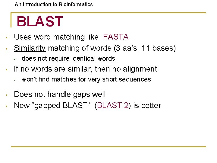
An Introduction to Bioinformatics BLAST • • Uses word matching like FASTA Similarity matching of words (3 aa’s, 11 bases) • • If no words are similar, then no alignment • • • does not require identical words. won’t find matches for very short sequences Does not handle gaps well New “gapped BLAST” (BLAST 2) is better

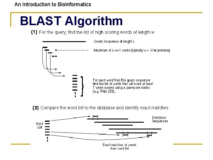
An Introduction to Bioinformatics BLAST Algorithm

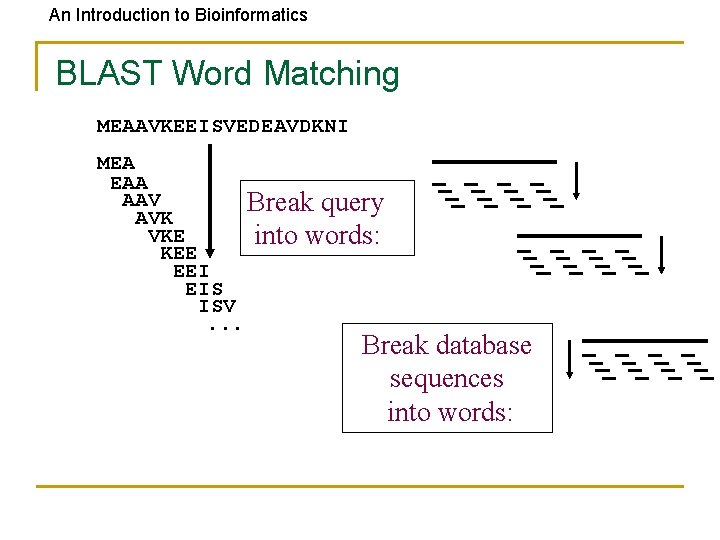
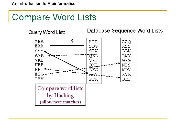
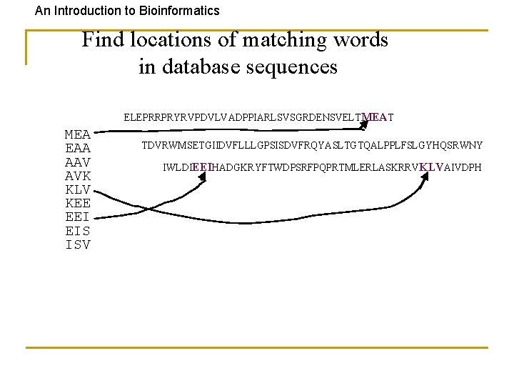
An Introduction to Bioinformatics BLAST Word Matching MEAAVKEEISVEDEAVDKNI MEA EAA AAV Break query AVK VKE into words: KEE EEI EIS ISV. . . Break database sequences into words:

An Introduction to Bioinformatics Compare Word Lists Database Sequence Word Lists Query Word List: MEA EAA AAV AVK VKL KEE EEI EIS ISV ? Compare word lists by Hashing (allow near matches) RTT SDG SRW QEL VKI DKI LFC AAV PFR … AAQ KSS LLN RWY GKG NIS WDV KVR DEI …

An Introduction to Bioinformatics Find locations of matching words in database sequences ELEPRRPRYRVPDVLVADPPIARLSVSGRDENSVELTMEAT MEA EAA AAV AVK KLV KEE EEI EIS ISV TDVRWMSETGIIDVFLLLGPSISDVFRQYASLTGTQALPPLFSLGYHQSRWNY IWLDIEEIHADGKRYFTWDPSRFPQPRTMLERLASKRRVKLVAIVDPH

An Introduction to Bioinformatics Extend hits one base at a time

An Introduction to Bioinformatics Seq_XYZ: Query: HVTGRSAF_FSYYGYGCYCGLGTGKGLPVDATDRCCWA QSVFDYIYYGCYCGWGLG_GK__PRDA E-val=10 -13 • Use two word matches as anchors to build an alignment between the query and a database sequence. • Then score the alignment.

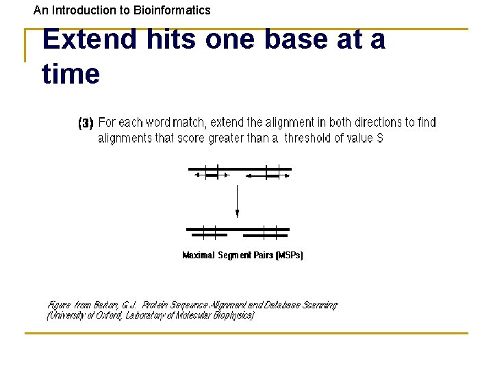
An Introduction to Bioinformatics HSPs are Aligned Regions • • The results of the word matching and attempts to extend the alignment are segments - called HSPs (High-scoring Segment Pairs) BLAST often produces several short HSPs rather than a single aligned region

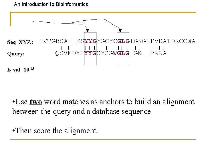
An Introduction to Bioinformatics BLAST 2 algorithm • The NCBI’s BLAST website now both use BLAST 2 (also known as “gapped BLAST”) • This algorithm is more complex than the original BLAST • It requires two word matches close to each other on a pair of sequences (i. e. with a gap) before it creates an alignment

An Introduction to Bioinformatics Statistical tests • Evaluate the probability of an event taking place by chance (at random). • P-value • • • Randomized data Distribution under the same setup Z-score • Chebyshev Inequality

An Introduction to Bioinformatics BLAST Statistics • E value is equivalent to standard P value (based on Karlin-Altschul theorem) • Significant if E < 0. 05 (smaller numbers are more significant) • The E-value represents the likelihood that the observed alignment is due to chance alone. A value of 1 indicates that an alignment this good would happen by chance with any random sequence searched against this database.

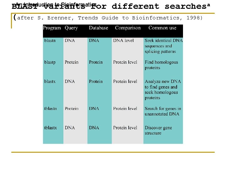
An Introduction to Bioinformatics BLAST variants for different searchesa (after S. Brenner, Trends Guide to Bioinformatics, 1998)

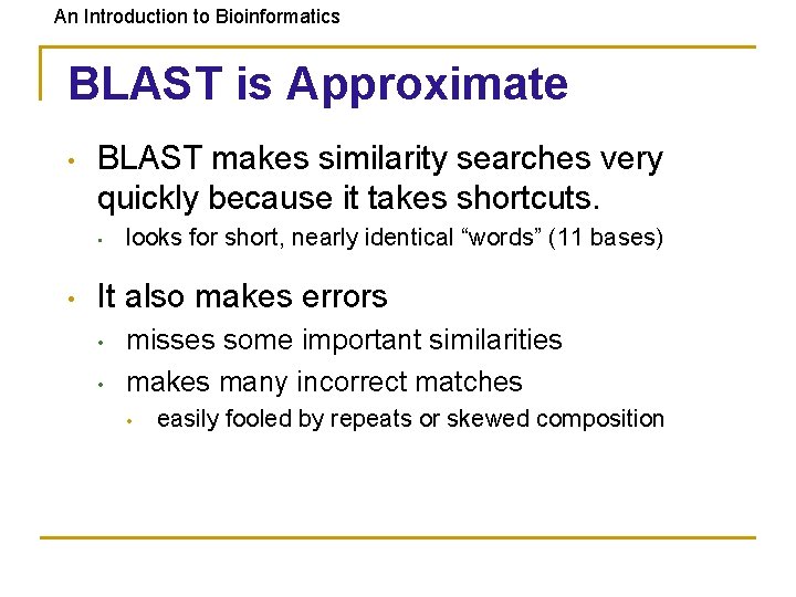
An Introduction to Bioinformatics BLAST is Approximate • BLAST makes similarity searches very quickly because it takes shortcuts. • • looks for short, nearly identical “words” (11 bases) It also makes errors • • misses some important similarities makes many incorrect matches • easily fooled by repeats or skewed composition

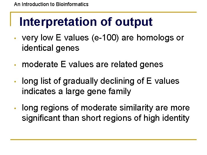
An Introduction to Bioinformatics Interpretation of output • very low E values (e-100) are homologs or identical genes • moderate E values are related genes • long list of gradually declining of E values indicates a large gene family • long regions of moderate similarity are more significant than short regions of high identity

An Introduction to Bioinformatics Biological Relevance • It is up to you, the biologist to scrutinize these alignments and determine if they are significant. • Were you looking for a short region of nearly identical sequence or a larger region of general similarity? • Are the mismatches conservative ones? • Are the matching regions important structural components of the genes or just introns and flanking regions?

An Introduction to Bioinformatics Borderline similarity • What to do with matches with E() values in the 0. 5 -1. 0 range? • this is the “Twilight Zone” • retest these sequences and look for related hits (not just your original query sequence) • similarity is transitive: if A~B and B~C, then A~C

An Introduction to Bioinformatics Position Specific Iterated BLAST • • Collect all database sequence segments that have been aligned with query sequence with Evalue below set threshold (default 0. 01) Construct position specific scoring matrix for collected sequences. Rough idea: • • Align all sequences to the query sequence as the template. Assign weights to the sequences Construct position specific scoring matrix Iterate

An Introduction to Bioinformatics Motif finding • Observation : Some regions have been better conserved than others during evolution • Idea: By analyzing the constant and variable properties of such groups of similar sequences, it is possible to derive a signature for a protein family or domain (motifs)

An Introduction to Bioinformatics PROSITE patterns • • PROSITE fingerprints are described by regular grammars There is a number of programs that allow to search databases for PROSITE patterns (example GCG package) Example [EDQH]-x-K-x-[DN]-G-x-R-[GACV] Rules: Each position is separated by a hyphen • One character denotes residuum at a given position • […] denoted a set of allowed residues • (n) denotes repeat of n • (n, m) denoted repeat between n and m inclusive Ex. ATP/GTP binding motive [SG]=X(4)-G-K-[DT] •

An Introduction to Bioinformatics Multiple sequence alignment

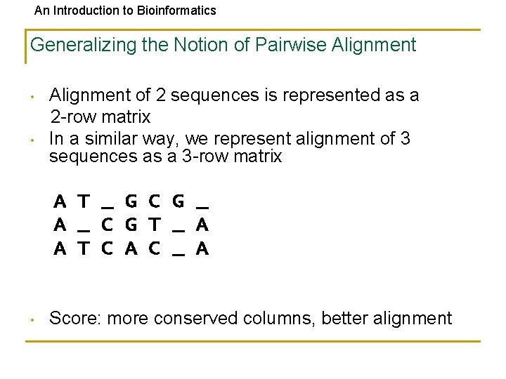
An Introduction to Bioinformatics Generalizing the Notion of Pairwise Alignment • • Alignment of 2 sequences is represented as a 2 -row matrix In a similar way, we represent alignment of 3 sequences as a 3 -row matrix A T _ G C G _ A _ C G T _ A A T C A C _ A • Score: more conserved columns, better alignment

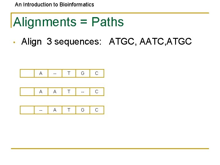
An Introduction to Bioinformatics Alignments = Paths • Align 3 sequences: ATGC, AATC, ATGC A -- T G C A A T -- C -- A T G C

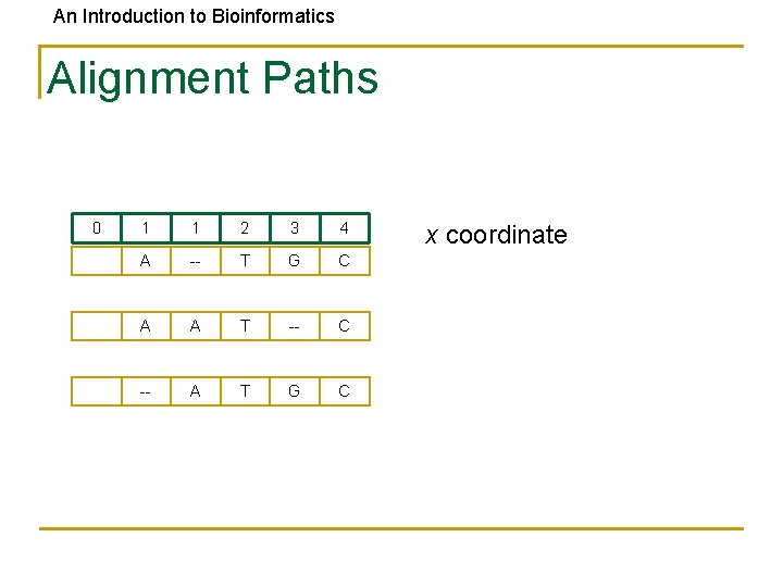
An Introduction to Bioinformatics Alignment Paths 0 1 1 2 3 4 A -- T G C A A T -- C -- A T G C x coordinate

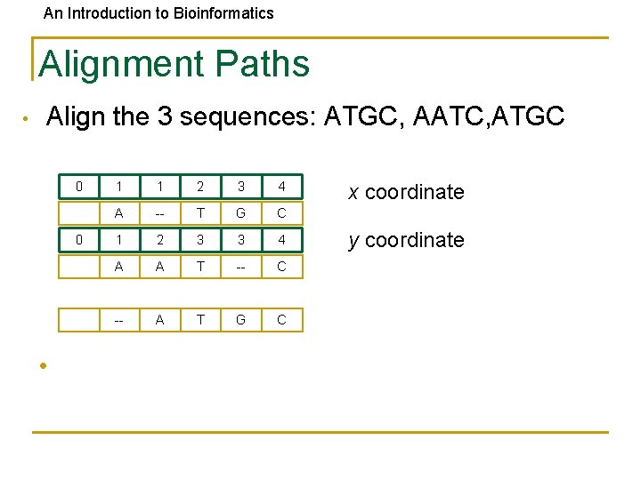
An Introduction to Bioinformatics Alignment Paths • Align the 3 sequences: ATGC, AATC, ATGC 0 0 • 1 1 2 3 4 A -- T G C 1 2 3 3 4 A A T -- C -- A T G C x coordinate y coordinate

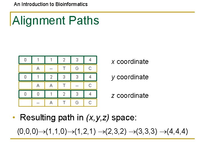
An Introduction to Bioinformatics Alignment Paths 0 0 0 1 1 2 3 4 A -- T G C 1 2 3 3 4 A A T -- C 0 1 2 3 4 -- A T G C x coordinate y coordinate z coordinate • Resulting path in (x, y, z) space: (0, 0, 0) (1, 1, 0) (1, 2, 1) (2, 3, 2) (3, 3, 3) (4, 4, 4)

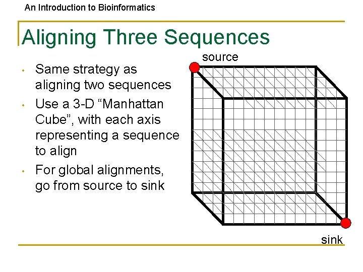
An Introduction to Bioinformatics Aligning Three Sequences • • • Same strategy as aligning two sequences Use a 3 -D “Manhattan Cube”, with each axis representing a sequence to align For global alignments, go from source to sink source sink

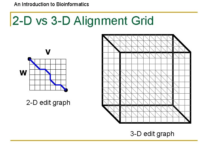
An Introduction to Bioinformatics 2 -D vs 3 -D Alignment Grid V W 2 -D edit graph 3 -D edit graph

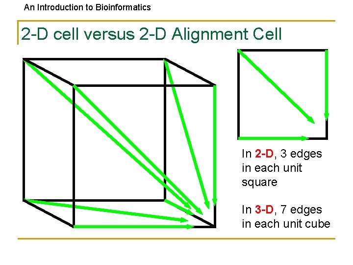
An Introduction to Bioinformatics 2 -D cell versus 2 -D Alignment Cell In 2 -D, 3 edges in each unit square In 3 -D, 7 edges in each unit cube

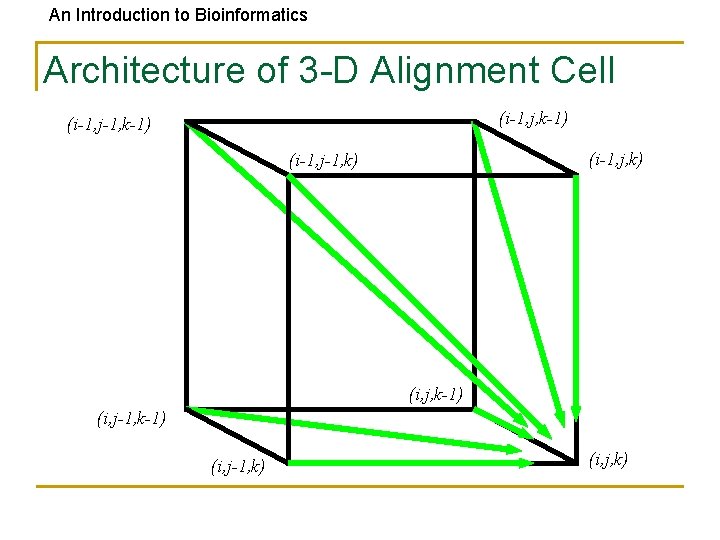
An Introduction to Bioinformatics Architecture of 3 -D Alignment Cell (i-1, j, k-1) (i-1, j-1, k-1) (i-1, j, k) (i-1, j-1, k) (i, j, k-1) (i, j-1, k) (i, j, k)

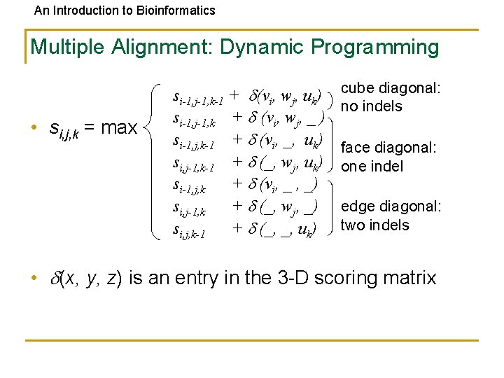
An Introduction to Bioinformatics Multiple Alignment: Dynamic Programming • si, j, k = max si-1, j-1, k-1 + (vi, wj, uk) si-1, j-1, k + (vi, wj, _ ) si-1, j, k-1 + (vi, _, uk) si, j-1, k-1 + (_, wj, uk) si-1, j, k + (vi, _ , _) si, j-1, k + (_, wj, _) si, j, k-1 + (_, _, uk) cube diagonal: no indels face diagonal: one indel edge diagonal: two indels • (x, y, z) is an entry in the 3 -D scoring matrix

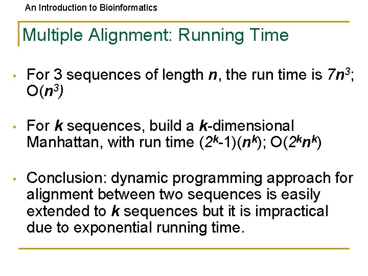
An Introduction to Bioinformatics Multiple Alignment: Running Time • For 3 sequences of length n, the run time is 7 n 3; O(n 3) • For k sequences, build a k-dimensional Manhattan, with run time (2 k-1)(nk); O(2 knk) • Conclusion: dynamic programming approach for alignment between two sequences is easily extended to k sequences but it is impractical due to exponential running time.

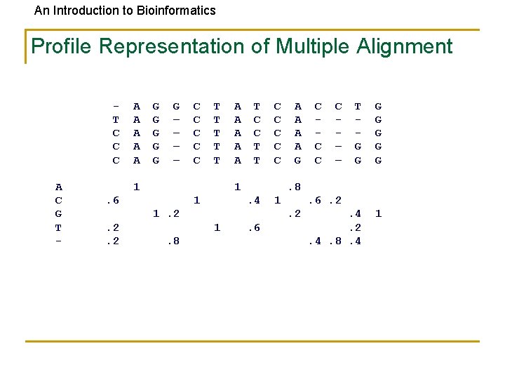
An Introduction to Bioinformatics Profile Representation of Multiple Alignment T C C C A C G T - A A A G G G – – C C C T T T 1 A A A T C C T T 1 . 6 1 . 4 1 C C – – T G G G G . 4. 2. 4. 8. 4 1 . 6. 2. 2 1. 8 A A G. 8 1. 2. 2. 2 C C C . 6

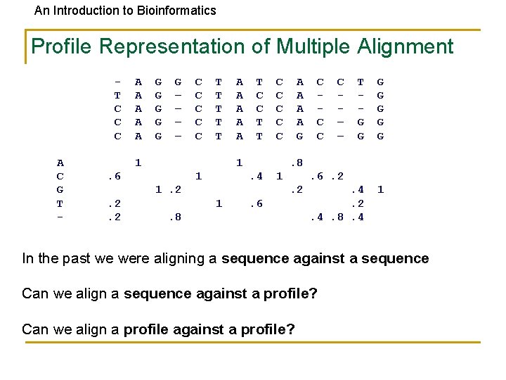
An Introduction to Bioinformatics Profile Representation of Multiple Alignment T C C C A C G T - A A A G G G – – C C C T T T 1 A A A T C C T T 1 . 6 1 A A G . 4 1 C – – T G G G G . 4. 2. 4. 8. 4 1 . 6. 2. 2 1 C C C . 8 1. 2. 2. 2 C C C . 6 . 8 In the past we were aligning a sequence against a sequence Can we align a sequence against a profile? Can we align a profile against a profile?

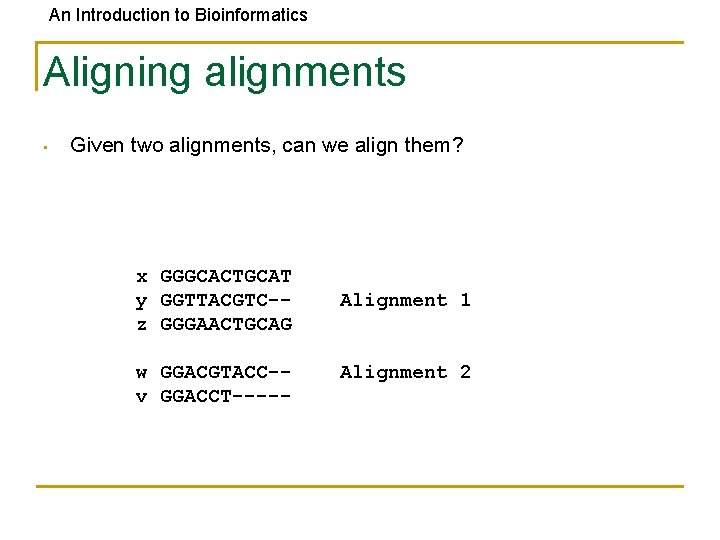
An Introduction to Bioinformatics Aligning alignments • Given two alignments, can we align them? x GGGCACTGCAT y GGTTACGTC-z GGGAACTGCAG w GGACGTACC-v GGACCT----- Alignment 1 Alignment 2

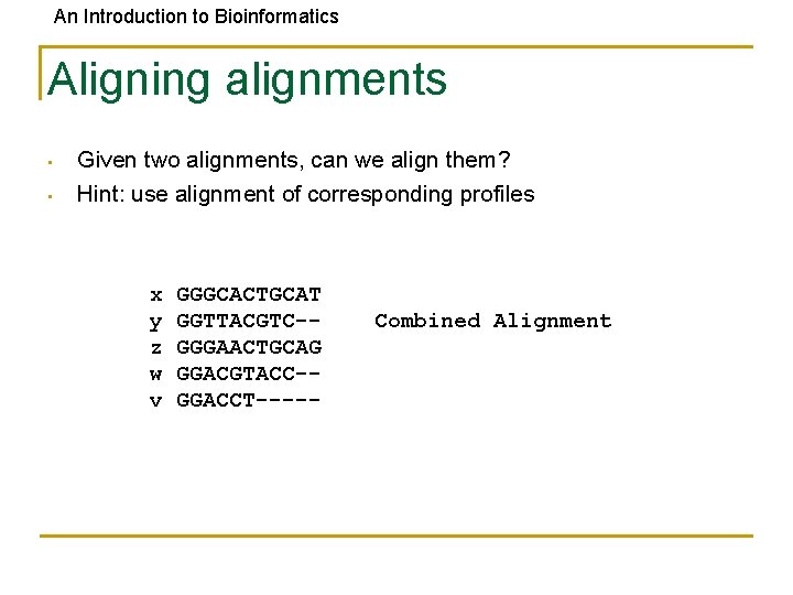
An Introduction to Bioinformatics Aligning alignments • • Given two alignments, can we align them? Hint: use alignment of corresponding profiles x y z w v GGGCACTGCAT GGTTACGTC-GGGAACTGCAG GGACGTACC-GGACCT----- Combined Alignment

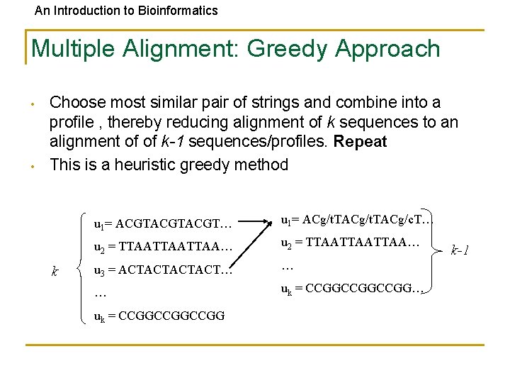
An Introduction to Bioinformatics Multiple Alignment: Greedy Approach • • Choose most similar pair of strings and combine into a profile , thereby reducing alignment of k sequences to an alignment of of k-1 sequences/profiles. Repeat This is a heuristic greedy method k u 1= ACGTACGT… u 1= ACg/t. TACg/c. T… u 2 = TTAATTAATTAA… u 3 = ACTACT… … … uk = CCGGCCGGCCGG k-1

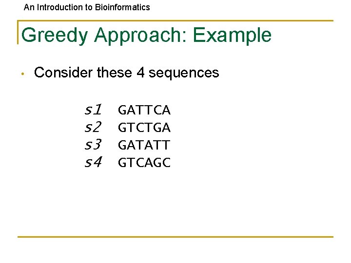
An Introduction to Bioinformatics Greedy Approach: Example • Consider these 4 sequences s 1 s 2 s 3 s 4 GATTCA GTCTGA GATATT GTCAGC

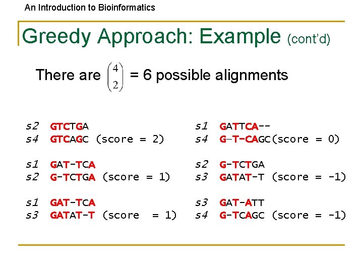
An Introduction to Bioinformatics Greedy Approach: Example (cont’d) • There are = 6 possible alignments s 2 s 4 GTCTGA GTCAGC (score = 2) s 1 s 4 GATTCA-G—T-CAGC(score = 0) s 1 s 2 GAT-TCA G-TCTGA (score = 1) s 2 s 3 G-TCTGA GATAT-T (score = -1) s 1 s 3 GAT-TCA GATAT-T (score s 3 s 4 GAT-ATT G-TCAGC (score = -1) = 1)

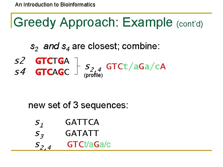
An Introduction to Bioinformatics Greedy Approach: Example (cont’d) s 2 and s 4 are closest; combine: s 2 s 4 GTCTGA GTCAGC s 2, 4 GTCt/a. Ga/c. A (profile) new set of 3 sequences: s 1 s 3 s 2, 4 GATTCA GATATT GTCt/a. Ga/c

An Introduction to Bioinformatics Progressive Alignment • • Progressive alignment is a variation of greedy algorithm with a somewhat more intelligent strategy for choosing the order of alignments. Progressive alignment works well for close sequences, but deteriorates for distant sequences • Gaps in consensus string are permanent • Use profiles to compare sequences

An Introduction to Bioinformatics Clustal. W • Popular multiple alignment tool today • ‘W’ stands for ‘weighted’ (different parts of alignment are weighted differently). • Three-step process 1. ) Construct pairwise alignments 2. ) Build Guide Tree 3. ) Progressive Alignment guided by the tree

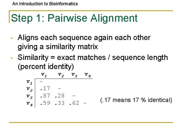
An Introduction to Bioinformatics Step 1: Pairwise Alignment • • Aligns each sequence again each other giving a similarity matrix Similarity = exact matches / sequence length (percent identity) v 1 v 2 v 3 v 4. 17. 87. 28. 59. 33. 62 - (. 17 means 17 % identical)

An Introduction to Bioinformatics Step 2: Guide Tree • Create Guide Tree using the similarity matrix • Clustal. W • Guide uses the neighbor-joining method tree roughly reflects evolutionary relations

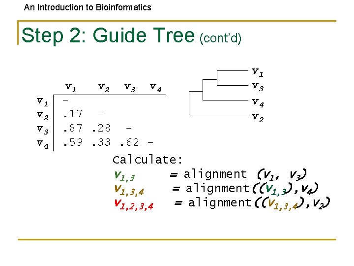
An Introduction to Bioinformatics Step 2: Guide Tree (cont’d) v 1 v 2 v 3 v 4. 17. 87. 28. 59. 33. 62 - v 1 v 3 v 4 v 2 Calculate: v 1, 3 = alignment (v 1, v 3) v 1, 3, 4 = alignment((v 1, 3), v 4) v 1, 2, 3, 4 = alignment((v 1, 3, 4), v 2)

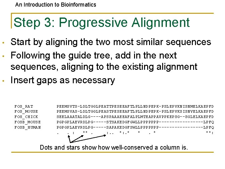
An Introduction to Bioinformatics Step 3: Progressive Alignment • • • Start by aligning the two most similar sequences Following the guide tree, add in the next sequences, aligning to the existing alignment Insert gaps as necessary FOS_RAT FOS_MOUSE FOS_CHICK FOSB_MOUSE FOSB_HUMAN PEEMSVTS-LDLTGGLPEATTPESEEAFTLPLLNDPEPK-PSLEPVKNISNMELKAEPFD PEEMSVAS-LDLTGGLPEASTPESEEAFTLPLLNDPEPK-PSLEPVKSISNVELKAEPFD SEELAAATALDLG----APSPAAAEEAFALPLMTEAPPAVPPKEPSG--SGLELKAEPFD PGPGPLAEVRDLPG-----STSAKEDGFGWLLPPPPPPP---------LPFQ PGPGPLAEVRDLPG-----SAPAKEDGFSWLLPPPPPPP---------LPFQ. . : **. : . . *: . * **: Dots and stars show well-conserved a column is.

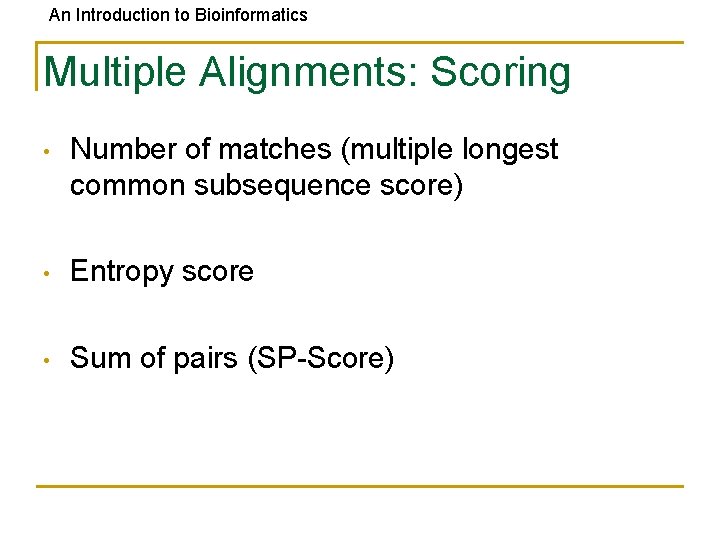
An Introduction to Bioinformatics Multiple Alignments: Scoring • Number of matches (multiple longest common subsequence score) • Entropy score • Sum of pairs (SP-Score)

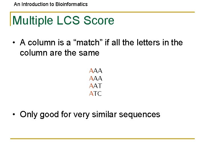
An Introduction to Bioinformatics Multiple LCS Score • A column is a “match” if all the letters in the column are the same AAA AAT ATC • Only good for very similar sequences

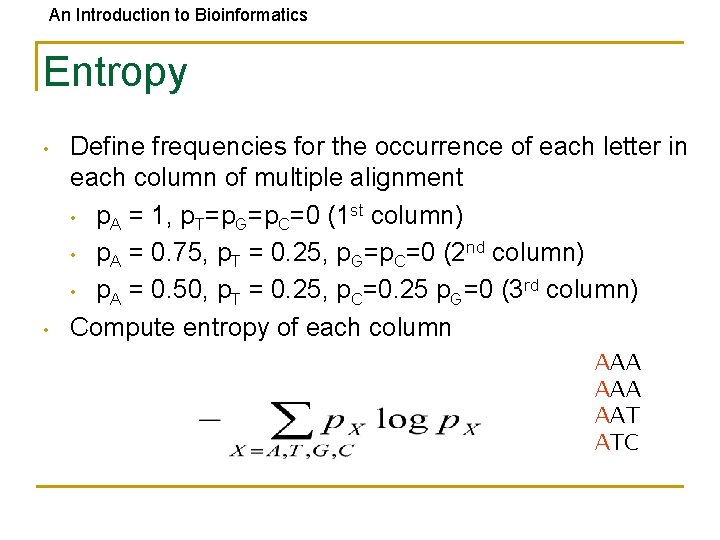
An Introduction to Bioinformatics Entropy • • Define frequencies for the occurrence of each letter in each column of multiple alignment • p. A = 1, p. T=p. G=p. C=0 (1 st column) • p. A = 0. 75, p. T = 0. 25, p. G=p. C=0 (2 nd column) • p. A = 0. 50, p. T = 0. 25, p. C=0. 25 p. G=0 (3 rd column) Compute entropy of each column AAA AAT ATC

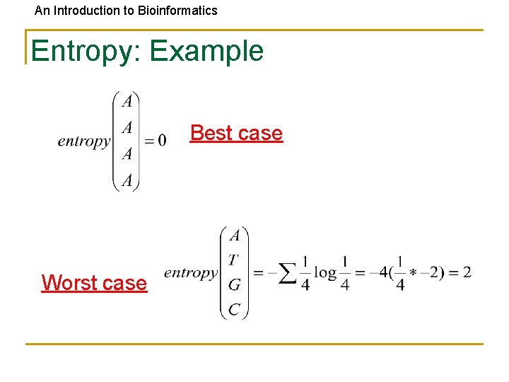
An Introduction to Bioinformatics Entropy: Example Best case Worst case

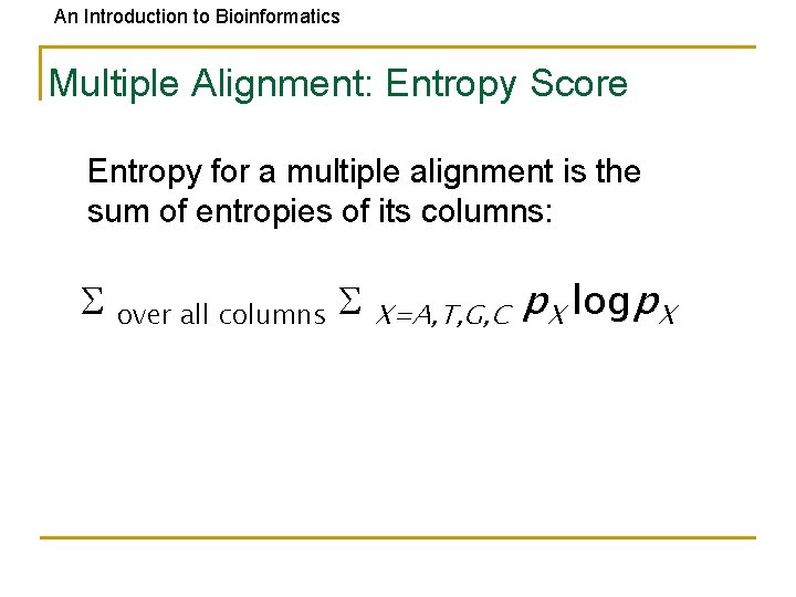
An Introduction to Bioinformatics Multiple Alignment: Entropy Score Entropy for a multiple alignment is the sum of entropies of its columns: over all columns X=A, T, G, C p. X logp. X

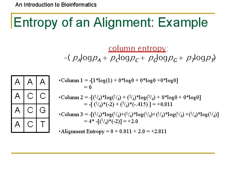
An Introduction to Bioinformatics Entropy of an Alignment: Example column entropy: -( p. Alogp. A + p. Clogp. C + p. Glogp. G + p. Tlogp. T) A A A • Column 1 = -[1*log(1) + 0*log 0 +0*log 0] =0 A C C • Column 2 = -[(1/4)*log(1/4) + (3/4)*log(3/4) + 0*log 0] = -[ (1/4)*(-2) + (3/4)*(-. 415) ] = +0. 811 A C G A C T • Column 3 = -[(1/4)*log(1/4)+(1/4)*log(1/4)] = 4* -[(1/4)*(-2)] = +2. 0 • Alignment Entropy = 0 + 0. 811 + 2. 0 = +2. 811

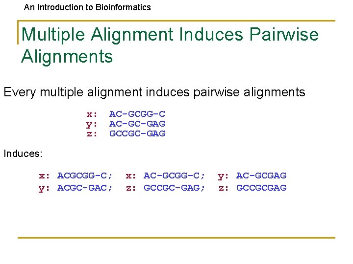
An Introduction to Bioinformatics Multiple Alignment Induces Pairwise Alignments Every multiple alignment induces pairwise alignments x: y: z: AC-GCGG-C AC-GC-GAG GCCGC-GAG Induces: x: ACGCGG-C; y: ACGC-GAC; x: AC-GCGG-C; z: GCCGC-GAG; y: AC-GCGAG z: GCCGCGAG

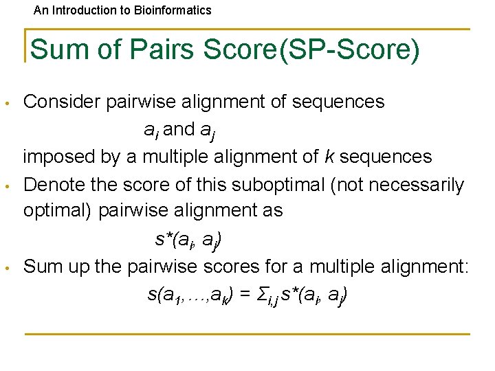
An Introduction to Bioinformatics Sum of Pairs Score(SP-Score) • • • Consider pairwise alignment of sequences ai and aj imposed by a multiple alignment of k sequences Denote the score of this suboptimal (not necessarily optimal) pairwise alignment as s*(ai, aj) Sum up the pairwise scores for a multiple alignment: s(a 1, …, ak) = Σi, j s*(ai, aj)

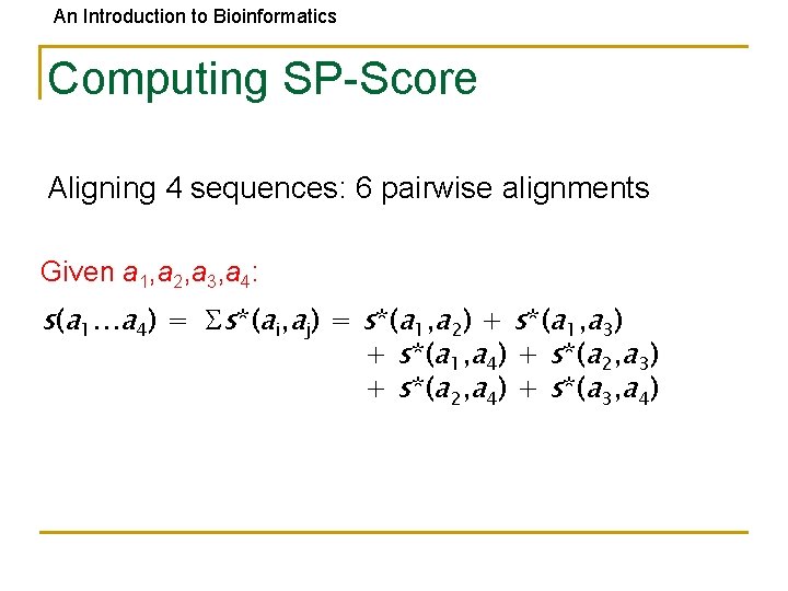
An Introduction to Bioinformatics Computing SP-Score Aligning 4 sequences: 6 pairwise alignments Given a 1, a 2, a 3, a 4: s(a 1…a 4) = s*(ai, aj) = s*(a 1, a 2) + s*(a 1, a 3) + s*(a 1, a 4) + s*(a 2, a 3) + s*(a 2, a 4) + s*(a 3, a 4)

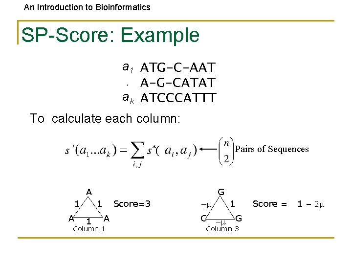
An Introduction to Bioinformatics SP-Score: Example a 1 ATG-C-AAT. A-G-CATAT ak ATCCCATTT To calculate each column: s Pairs of Sequences s*( A 1 A G 1 1 Score=3 A Column 1 1 -m C -m G Column 3 Score = 1 – 2 m

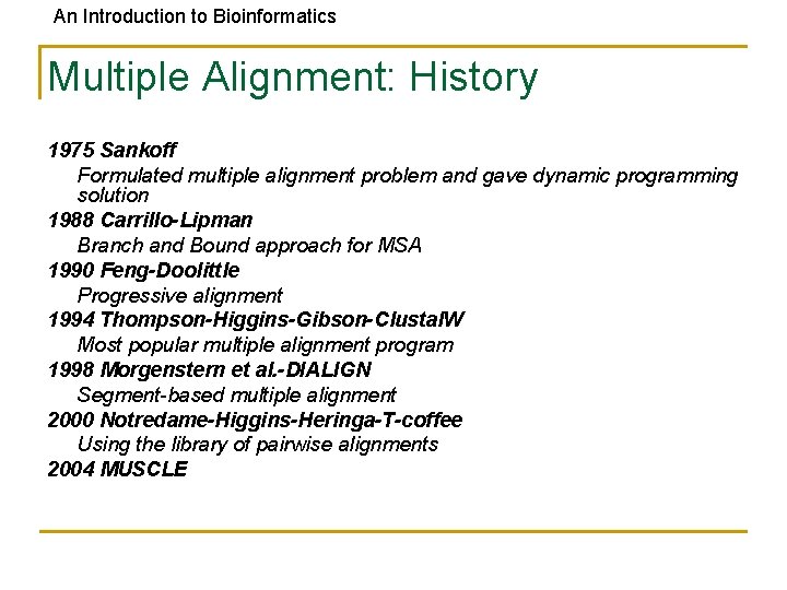
An Introduction to Bioinformatics Multiple Alignment: History 1975 Sankoff Formulated multiple alignment problem and gave dynamic programming solution 1988 Carrillo-Lipman Branch and Bound approach for MSA 1990 Feng-Doolittle Progressive alignment 1994 Thompson-Higgins-Gibson-Clustal. W Most popular multiple alignment program 1998 Morgenstern et al. -DIALIGN Segment-based multiple alignment 2000 Notredame-Higgins-Heringa-T-coffee Using the library of pairwise alignments 2004 MUSCLE