An introduction to Bayesian inference and model comparison
An introduction to Bayesian inference and model comparison J. Daunizeau ICM, Paris, France TNU, Zurich, Switzerland
Overview of the talk ü An introduction to probabilistic modelling ü Bayesian model comparison ü SPM applications
Overview of the talk ü An introduction to probabilistic modelling ü Bayesian model comparison ü SPM applications
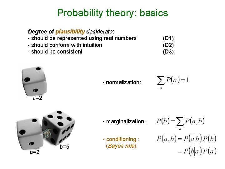
Probability theory: basics Degree of plausibility desiderata: - should be represented using real numbers - should conform with intuition - should be consistent • normalization: a=2 • marginalization: a=2 b=5 • conditioning : (Bayes rule) (D 1) (D 2) (D 3)
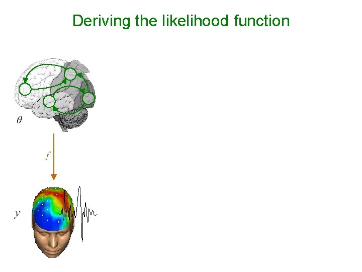
Deriving the likelihood function - Model of data with unknown parameters: e. g. , GLM: - But data is noisy: - Assume noise/residuals is ‘small’: f → Distribution of data, given fixed parameters:
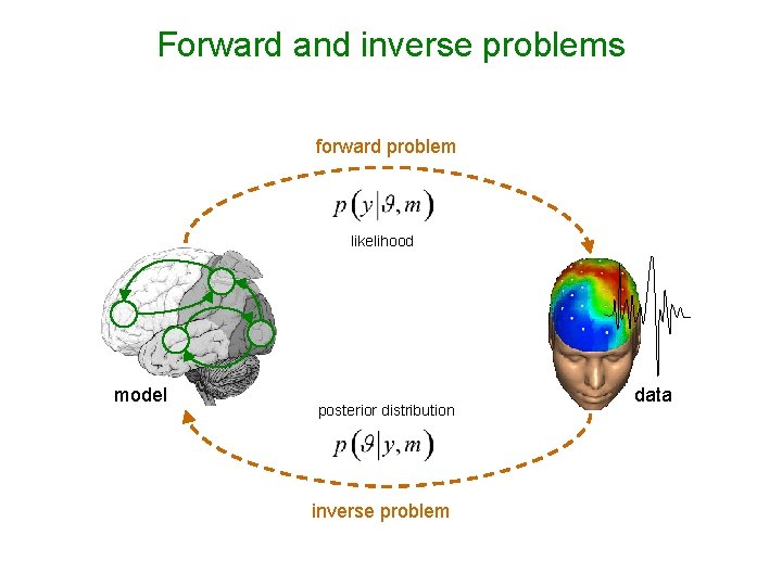
Forward and inverse problems forward problem likelihood model posterior distribution inverse problem data
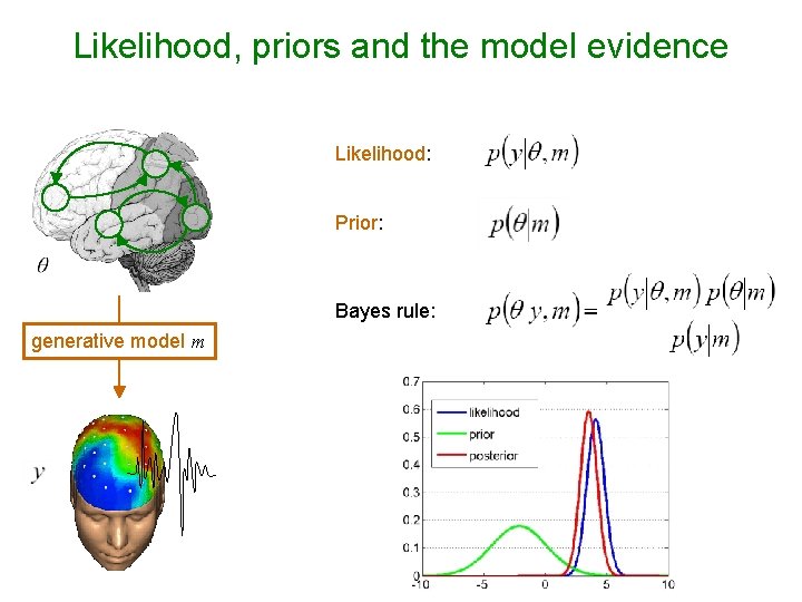
Likelihood, priors and the model evidence Likelihood: Prior: Bayes rule: generative model m
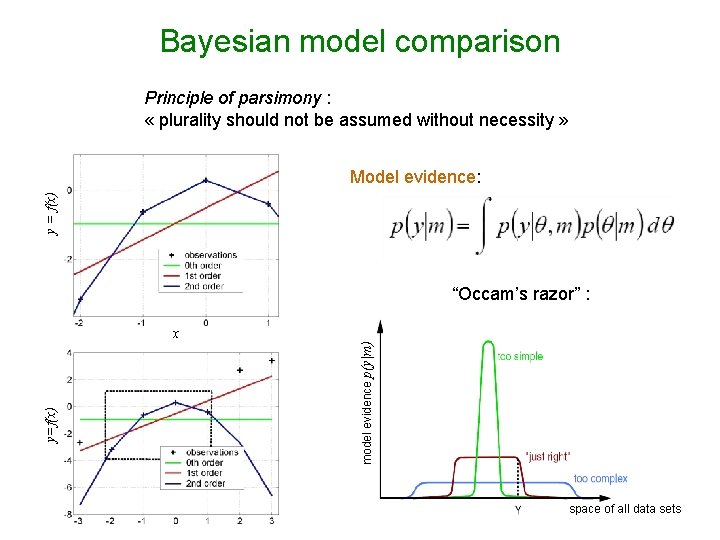
Bayesian model comparison Principle of parsimony : « plurality should not be assumed without necessity » y = f(x) Model evidence: “Occam’s razor” : model evidence p(y|m) y=f(x) x space of all data sets
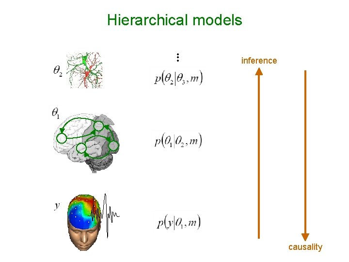
Hierarchical models • • • inference causality
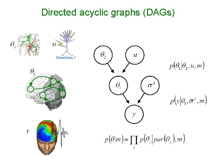
Directed acyclic graphs (DAGs)
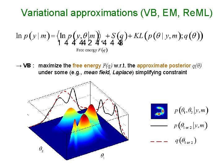
Variational approximations (VB, EM, Re. ML) → VB : maximize the free energy F(q) w. r. t. the approximate posterior q(θ) under some (e. g. , mean field, Laplace) simplifying constraint
Type, role and impact of priors • Types of priors: ü Explicit priors on model parameters (e. g. , Gaussian) ü Implicit priors on model functional form (e. g. , evolution & observation functions) ü Choice of “interesting” data features (e. g. , response magnitude vs response prof • Role of explicit priors (on model parameters): ü Resolving the ill-posedness of the inverse problem ü Avoiding overfitting (cf. generalization error) • Impact of priors: ü On parameter posterior distributions (cf. “shrinkage to the mean” effect) ü On model evidence (cf. “Occam’s razor”)
Overview of the talk ü An introduction to probabilistic modelling ü Bayesian model comparison ü SPM applications
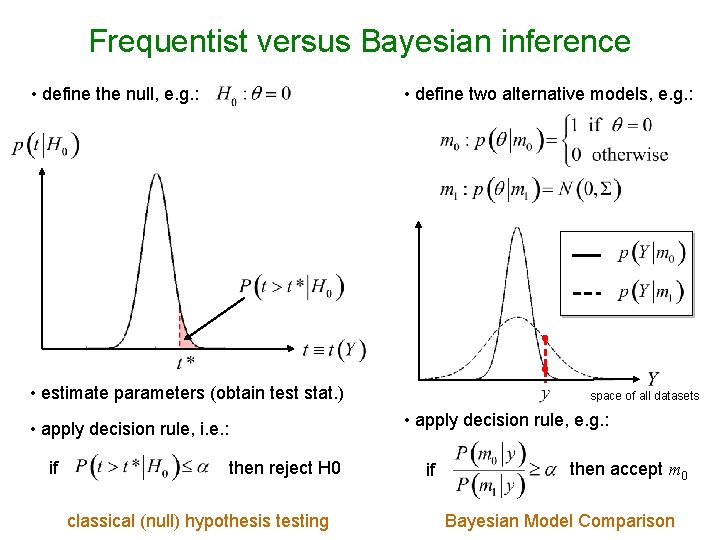
Frequentist versus Bayesian inference • define two alternative models, e. g. : • define the null, e. g. : • estimate parameters (obtain test stat. ) • apply decision rule, e. g. : • apply decision rule, i. e. : if space of all datasets then reject H 0 classical (null) hypothesis testing if then accept m 0 Bayesian Model Comparison
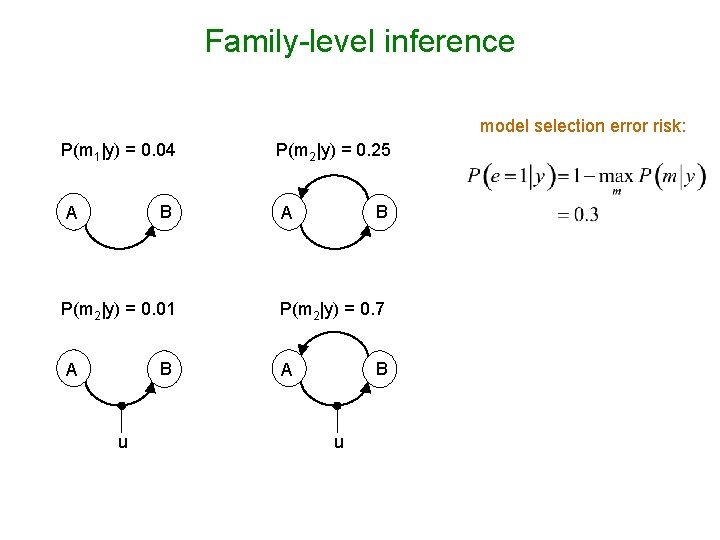
Family-level inference model selection error risk: P(m 1|y) = 0. 04 B A P(m 2|y) = 0. 01 B A u P(m 2|y) = 0. 25 B A P(m 2|y) = 0. 7 B A u
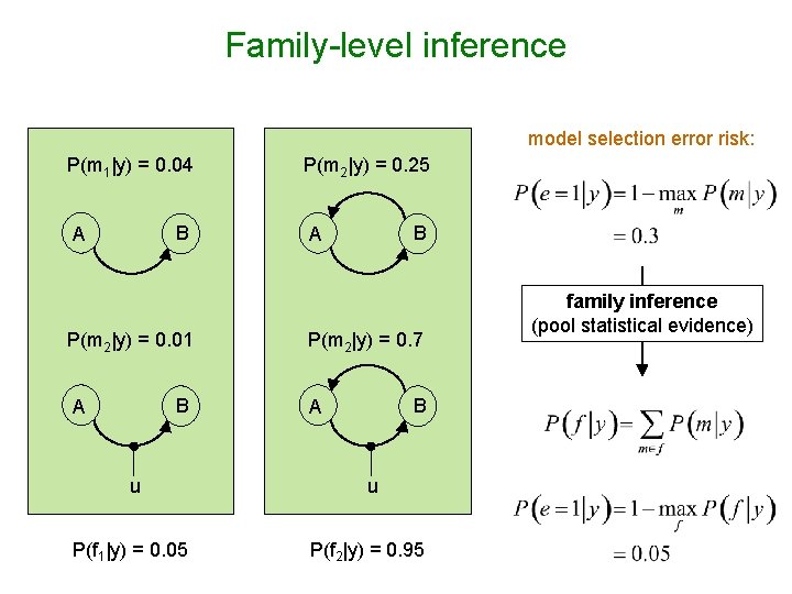
Family-level inference model selection error risk: P(m 1|y) = 0. 04 B A P(m 2|y) = 0. 01 B A P(m 2|y) = 0. 25 B A P(m 2|y) = 0. 7 B A u u P(f 1|y) = 0. 05 P(f 2|y) = 0. 95 family inference (pool statistical evidence)
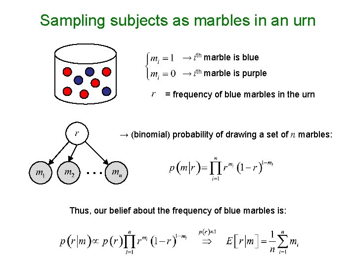
Sampling subjects as marbles in an urn → ith marble is blue → ith marble is purple = frequency of blue marbles in the urn → (binomial) probability of drawing a set of n marbles: … Thus, our belief about the frequency of blue marbles is:
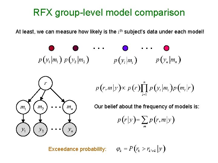
RFX group-level model comparison At least, we can measure how likely is the ith subject’s data under each model! … … … Our belief about the frequency of models is: … Exceedance probability:
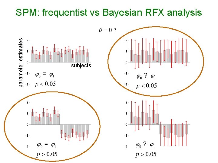
parameter estimates SPM: frequentist vs Bayesian RFX analysis subjects
Overview of the talk ü An introduction to probabilistic modelling ü Bayesian model comparison ü SPM applications
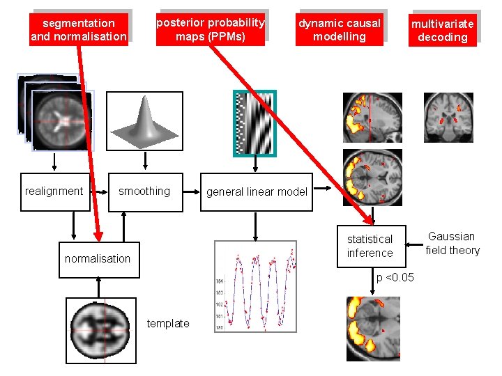
segmentation and normalisation realignment posterior probability maps (PPMs) smoothing dynamic causal modelling multivariate decoding general linear model statistical inference normalisation p <0. 05 template Gaussian field theory
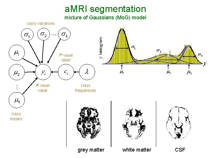
a. MRI segmentation mixture of Gaussians (Mo. G) model class variances … … ith voxel label ith voxel value class frequencies class means grey matter white matter CSF
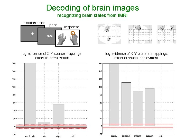
Decoding of brain images recognizing brain states from f. MRI fixation cross + pace response >> log-evidence of X-Y sparse mappings: effect of lateralization log-evidence of X-Y bilateral mappings: effect of spatial deployment
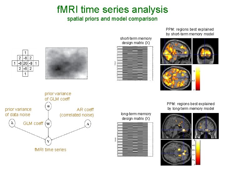
f. MRI time series analysis spatial priors and model comparison PPM: regions best explained by short-term memory model short-term memory design matrix (X) prior variance of GLM coeff prior variance of data noise AR coeff (correlated noise) GLM coeff f. MRI time series PPM: regions best explained by long-term memory model long-term memory design matrix (X)
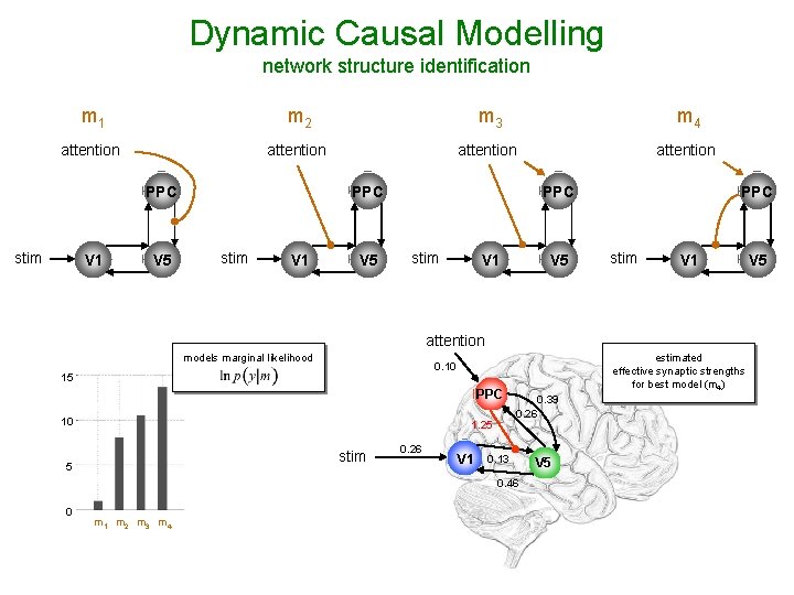
Dynamic Causal Modelling network structure identification m 1 m 2 m 3 m 4 attention PPC stim V 1 V 5 PPC stim V 1 attention models marginal likelihood 15 PPC 10 1. 25 stim 5 estimated effective synaptic strengths for best model (m 4) 0. 10 0. 26 V 1 0. 39 0. 26 0. 13 0. 46 0 m 1 m 2 m 3 m 4 V 5

I thank you for your attention.
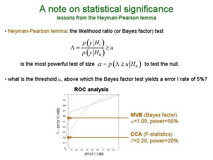
A note on statistical significance lessons from the Neyman-Pearson lemma • Neyman-Pearson lemma: the likelihood ratio (or Bayes factor) test is the most powerful test of size to test the null. • what is the threshold u, above which the Bayes factor test yields a error I rate of 5%? 1 - error II rate ROC analysis MVB (Bayes factor) u=1. 09, power=56% CCA (F-statistics) F=2. 20, power=20% error I rate
- Slides: 27