An Introduction to Artificial Intelligence Lecture 3 Solving

An Introduction to Artificial Intelligence Lecture 3: Solving Problems by Sorting Ramin Halavati (halavati@ce. sharif. edu) In which we look at how an agent can decide what to do by systematically considering the outcomes of various sequences of actions that it might take.

Outline • • • Problem-solving agents (Goal Based( Problem types Problem formulation Example problems Basic search algorithms

Assumptions • World States • Actions as transitions between states • Goal Formulation: A set of states • Problem Formulation: – The sequence of required actions to move from current state to a goal state

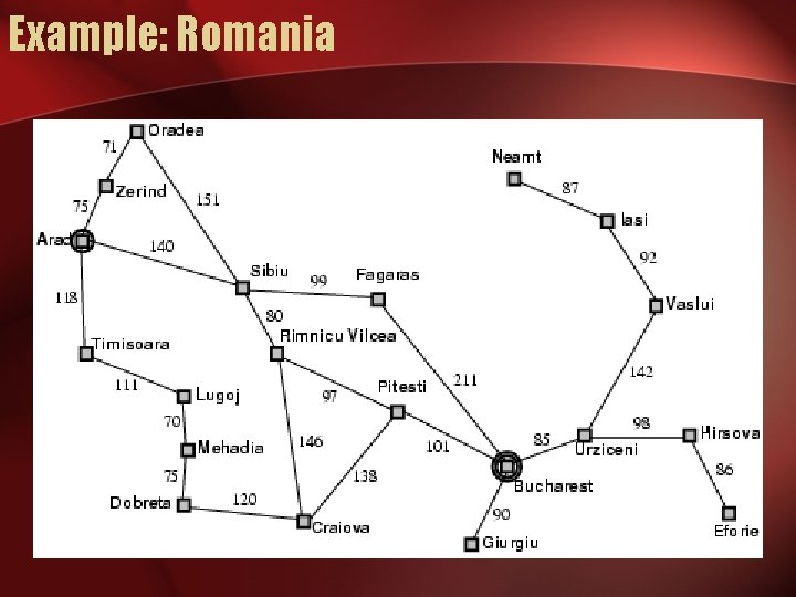
Example: Romania • On holiday in Romania; currently in Arad. • Flight leaves tomorrow from Bucharest • Formulate goal: – be in Bucharest • Formulate problem: – states: various cities – actions: drive between cities • Find solution: – sequence of cities, e. g. , Arad, Sibiu, Fagaras, Bucharest

Example: Romania

Setting the scene… • Problem solving by searching – Tree of possible actions sequences. • Knowledge is Power! – States – State transfers

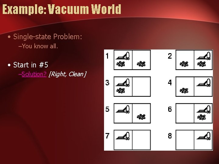
Example: Vacuum World • Single-state Problem: –You know all. • Start in #5 –Solution? [Right, Clean]

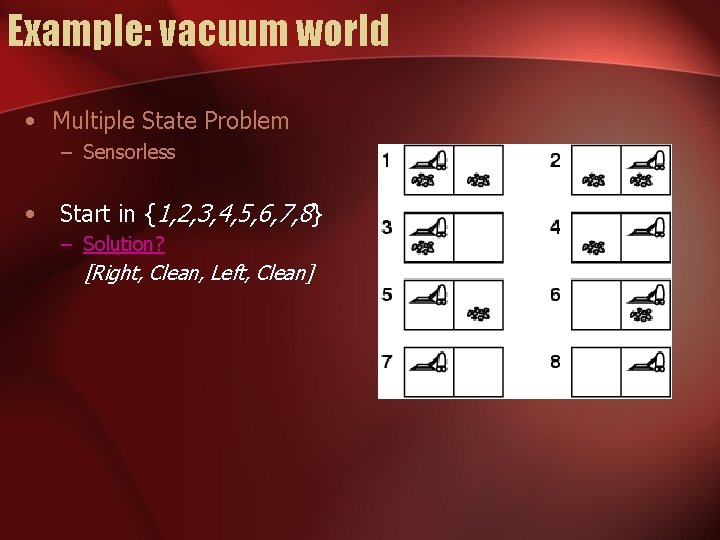
Example: vacuum world • Multiple State Problem – Sensorless • Start in {1, 2, 3, 4, 5, 6, 7, 8} – Solution? [Right, Clean, Left, Clean]

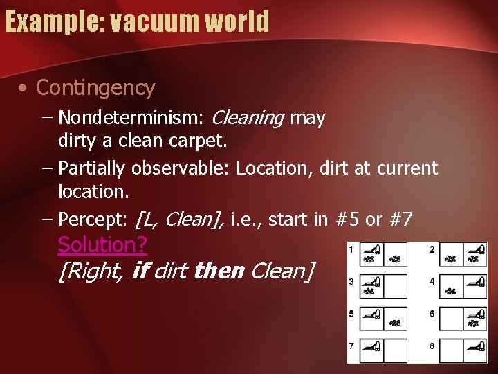
Example: vacuum world • Contingency – Nondeterminism: Cleaning may dirty a clean carpet. – Partially observable: Location, dirt at current location. – Percept: [L, Clean], i. e. , start in #5 or #7 Solution? [Right, if dirt then Clean]

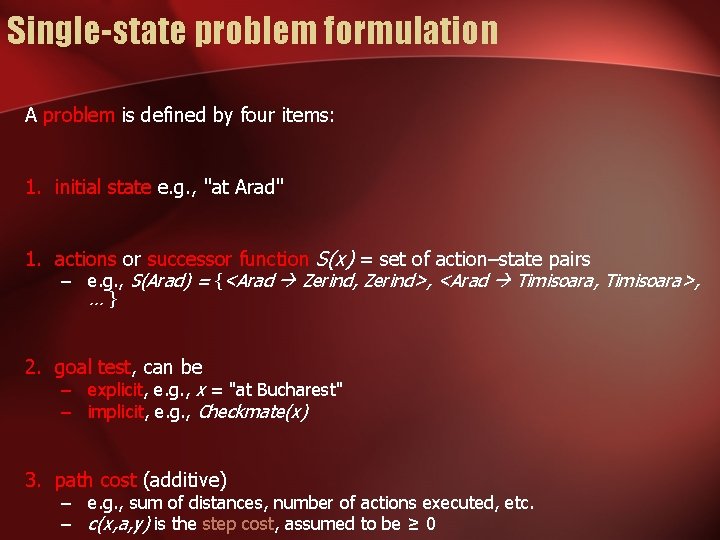
Single-state problem formulation A problem is defined by four items: 1. initial state e. g. , "at Arad" 1. actions or successor function S(x) = set of action–state pairs – e. g. , S(Arad) = {<Arad Zerind, Zerind>, <Arad Timisoara, Timisoara>, …} 2. goal test, can be – explicit, e. g. , x = "at Bucharest" – implicit, e. g. , Checkmate(x) 3. path cost (additive) – e. g. , sum of distances, number of actions executed, etc. – c(x, a, y) is the step cost, assumed to be ≥ 0

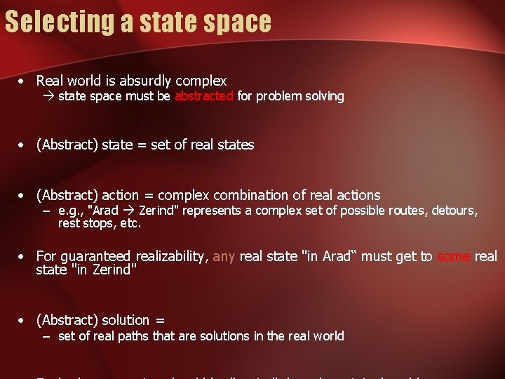
Selecting a state space • Real world is absurdly complex state space must be abstracted for problem solving • (Abstract) state = set of real states • (Abstract) action = complex combination of real actions – e. g. , "Arad Zerind" represents a complex set of possible routes, detours, rest stops, etc. • For guaranteed realizability, any real state "in Arad“ must get to some real state "in Zerind" • (Abstract) solution = – set of real paths that are solutions in the real world

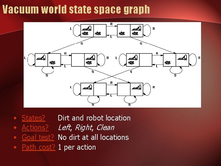
Vacuum world state space graph • • States? Actions? Goal test? Path cost? Dirt and robot location Left, Right, Clean No dirt at all locations 1 per action

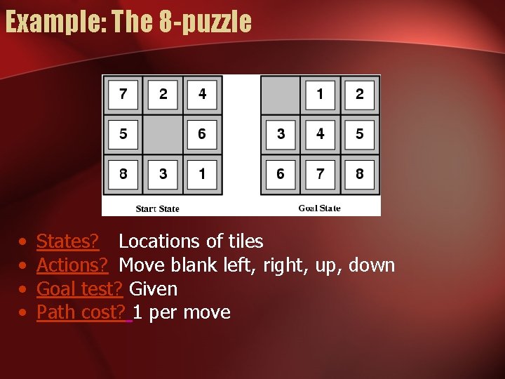
Example: The 8 -puzzle • • States? Locations of tiles Actions? Move blank left, right, up, down Goal test? Given Path cost? 1 per move

Example: robotic assembly • States? real-valued coordinates of robot joint angles parts of the object to be assembled • Actions? continuous motions of robot joints • Goal test? complete assembly

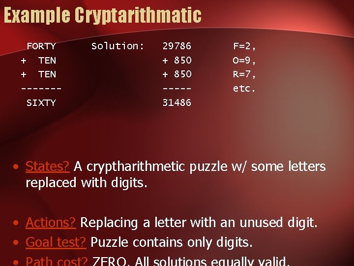
Example Cryptarithmatic FORTY + TEN ------SIXTY Solution: 29786 + 850 ----31486 F=2, O=9, R=7, etc. • States? A cryptharithmetic puzzle w/ some letters replaced with digits. • Actions? Replacing a letter with an unused digit. • Goal test? Puzzle contains only digits.

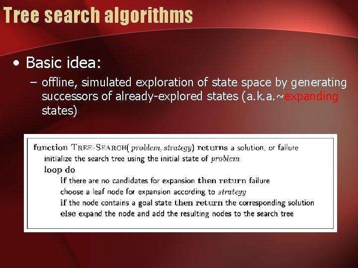
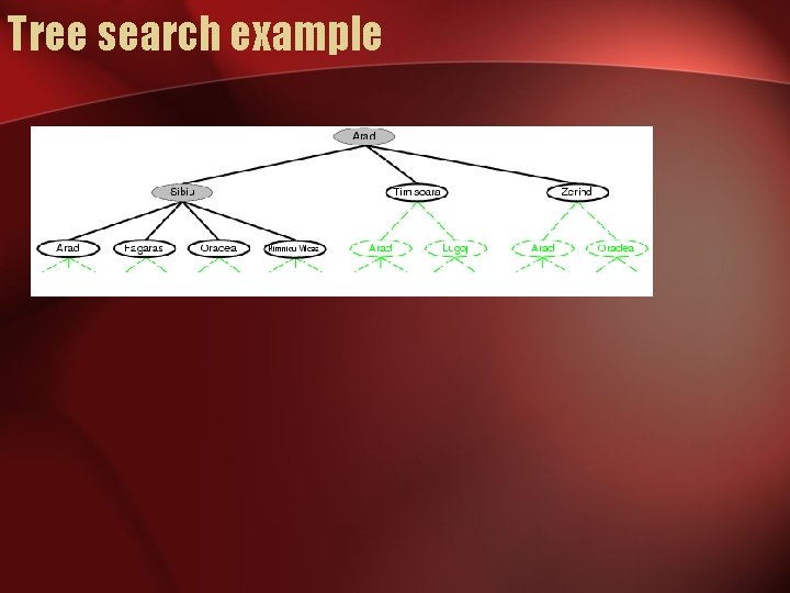
Tree search algorithms • Basic idea: – offline, simulated exploration of state space by generating successors of already-explored states (a. k. a. ~expanding states)

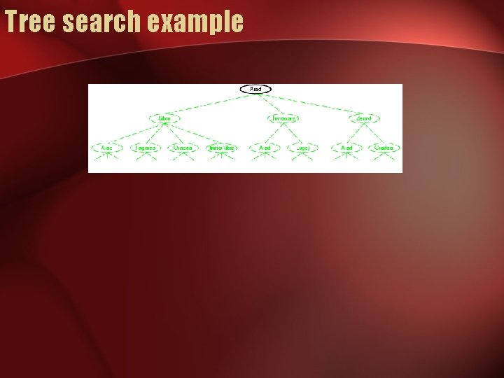
Tree search example

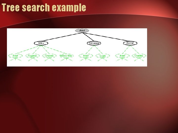
Tree search example

Tree search example

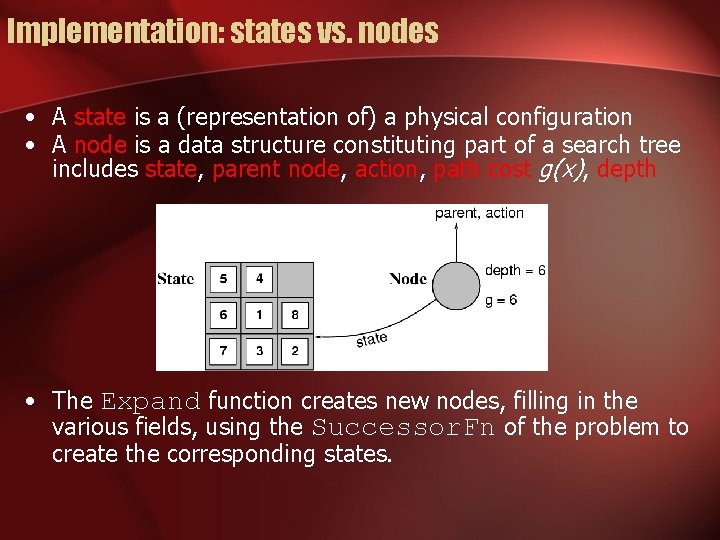
Implementation: states vs. nodes • A state is a (representation of) a physical configuration • A node is a data structure constituting part of a search tree includes state, parent node, action, path cost g(x), depth • The Expand function creates new nodes, filling in the various fields, using the Successor. Fn of the problem to create the corresponding states.

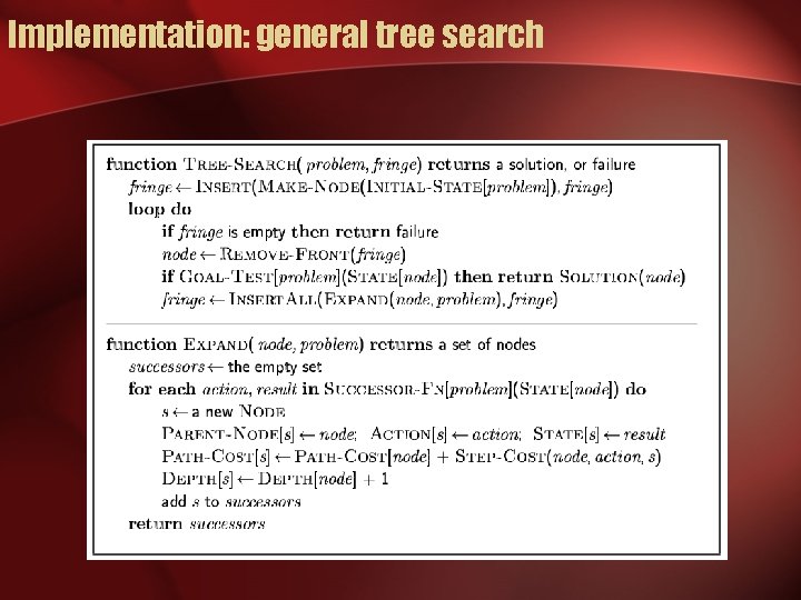
Implementation: general tree search

Search strategies • A search strategy is defined by picking the order of node expansion • Strategies are evaluated along the following dimensions: – – completeness: does it always find a solution if one exists? time complexity: number of nodes generated space complexity: maximum number of nodes in memory optimality: does it always find a least-cost solution? • Time and space complexity are measured in terms of – b: maximum branching factor of the search tree – d: depth of the least-cost solution – m: maximum depth of the state space (may be ∞)

Uninformed search strategies • Uninformed search strategies use only the information available in the problem definition – Breadth-first search – Uniform-cost search – Depth-first search

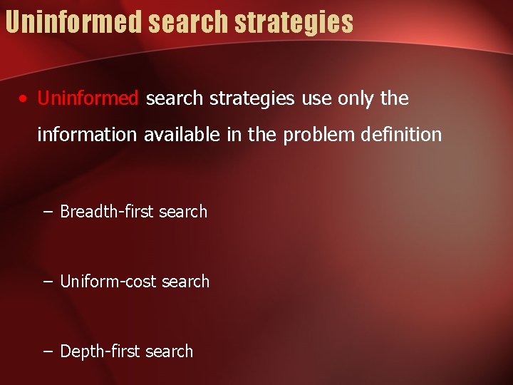
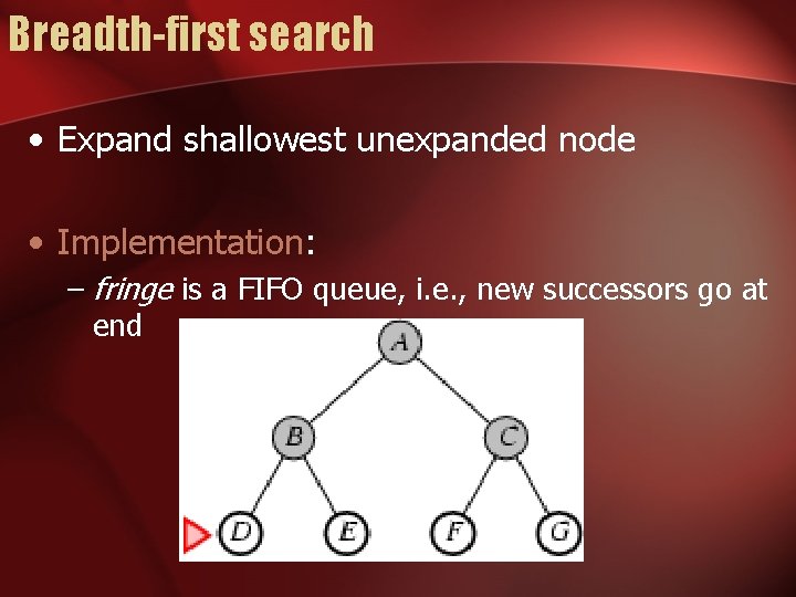
Breadth-first search • Expand shallowest unexpanded node • Implementation: – fringe is a FIFO queue, i. e. , new successors go at end

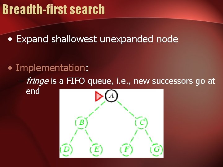
Breadth-first search • Expand shallowest unexpanded node • Implementation: –fringe is a FIFO queue, i. e. , new successors go at end

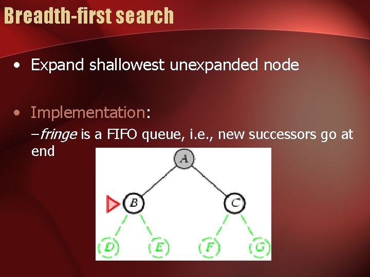
Breadth-first search • Expand shallowest unexpanded node • Implementation: – fringe is a FIFO queue, i. e. , new successors go at end

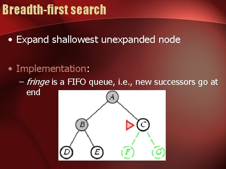
Breadth-first search • Expand shallowest unexpanded node • Implementation: – fringe is a FIFO queue, i. e. , new successors go at end

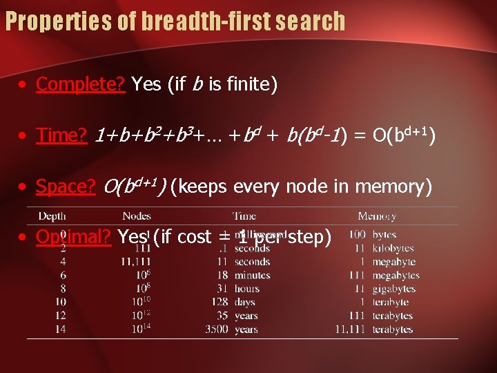
Properties of breadth-first search • Complete? Yes (if b is finite) • Time? 1+b+b 2+b 3+… +bd + b(bd-1) = O(bd+1) • Space? O(bd+1) (keeps every node in memory) • Optimal? Yes (if cost = 1 per step)

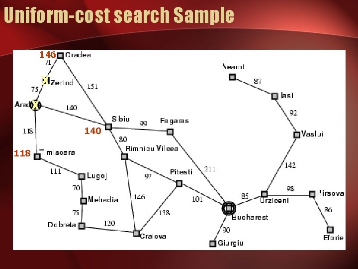
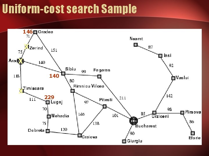
Uniform-cost search • Expand least-cost unexpanded node • Implementation: – fringe = queue ordered by path cost • Equivalent to breadth-first if step costs all equal

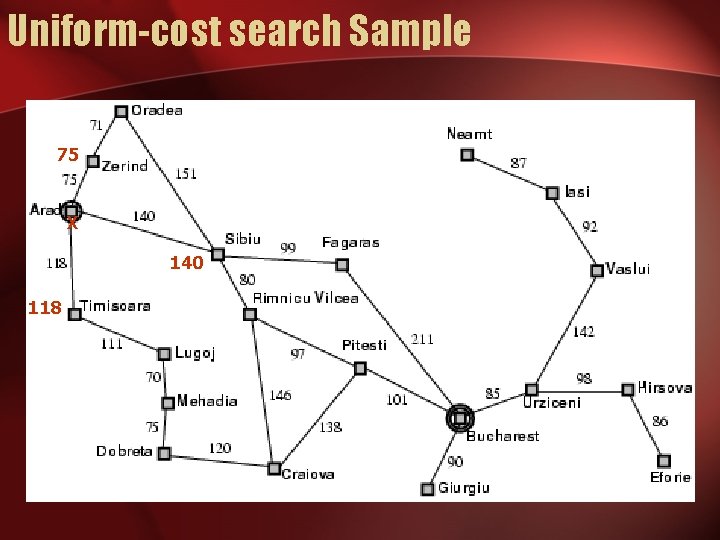
Uniform-cost search Sample 0

Uniform-cost search Sample 75 X 140 118

Uniform-cost search Sample 146 X X 140 118

Uniform-cost search Sample 146 X X 140 X 229

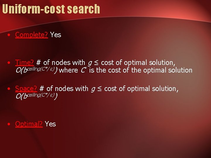
Uniform-cost search • Complete? Yes • Time? # of nodes with g ≤ cost of optimal solution, O(bceiling(C*/ ε)) where C* is the cost of the optimal solution • Space? # of nodes with g ≤ cost of optimal solution, O(bceiling(C*/ ε)) • Optimal? Yes

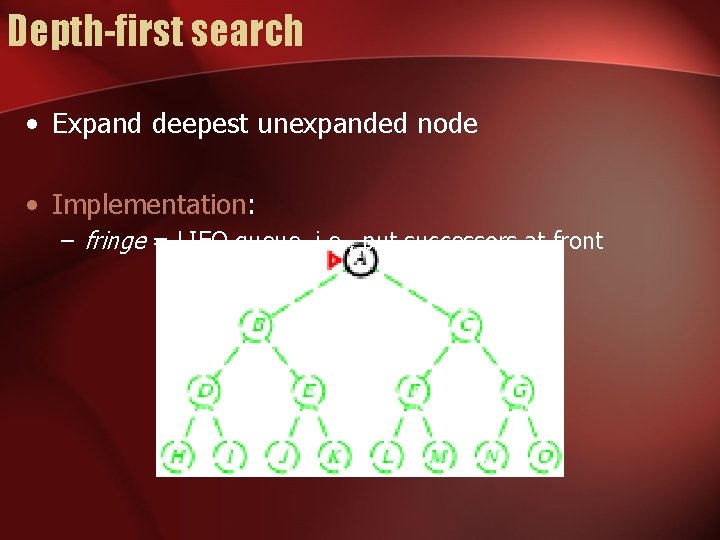
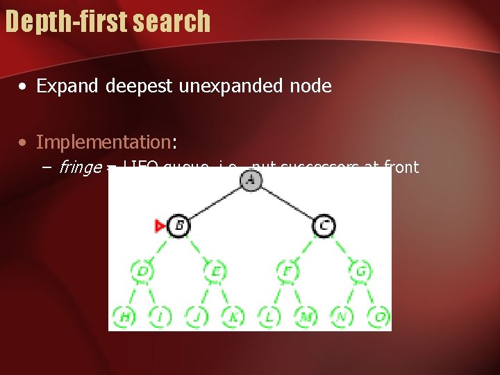
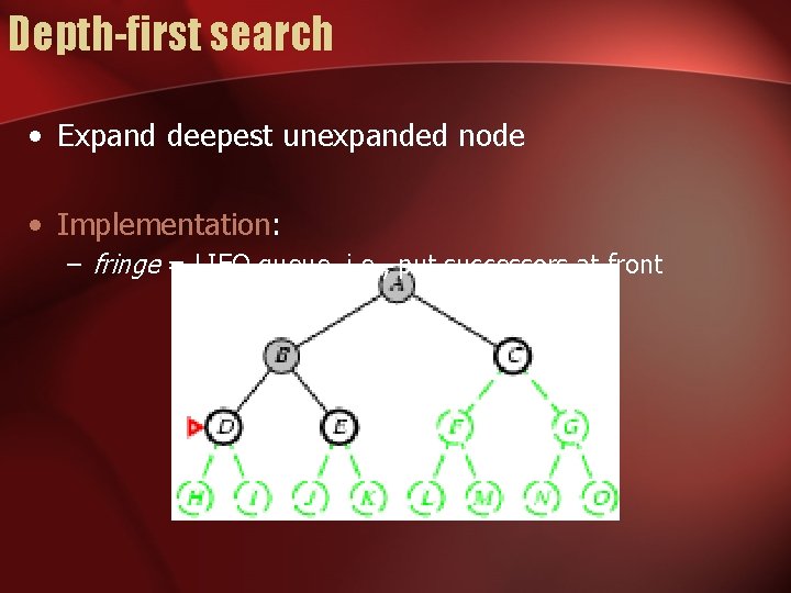
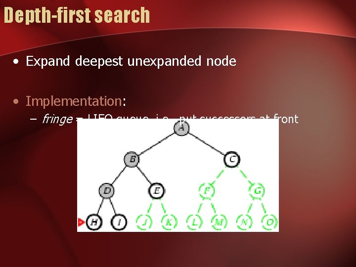
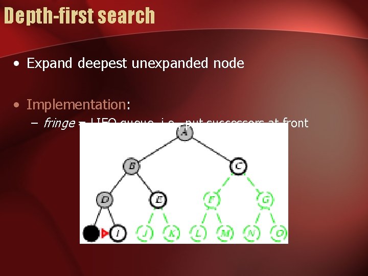
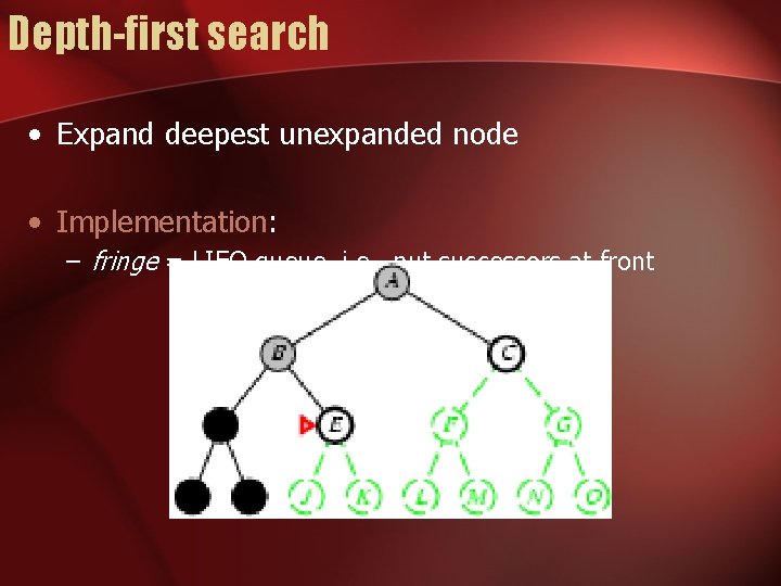
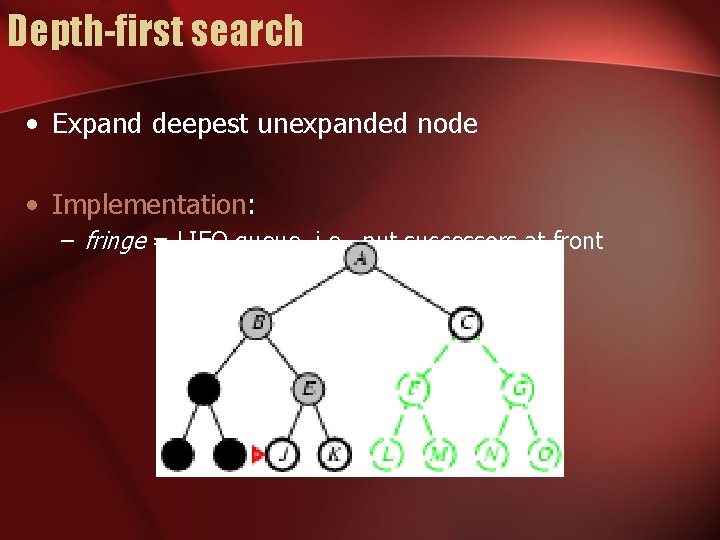
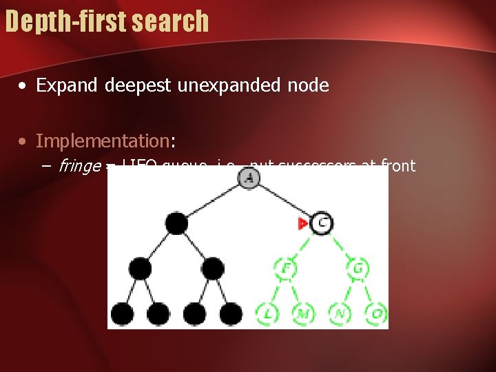
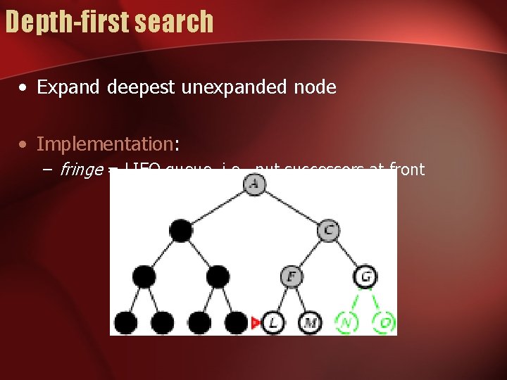
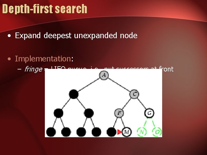
Depth-first search • Expand deepest unexpanded node • Implementation: – fringe = LIFO queue, i. e. , put successors at front

Depth-first search • Expand deepest unexpanded node • Implementation: – fringe = LIFO queue, i. e. , put successors at front

Depth-first search • Expand deepest unexpanded node • Implementation: – fringe = LIFO queue, i. e. , put successors at front

Depth-first search • Expand deepest unexpanded node • Implementation: – fringe = LIFO queue, i. e. , put successors at front

Depth-first search • Expand deepest unexpanded node • Implementation: – fringe = LIFO queue, i. e. , put successors at front

Depth-first search • Expand deepest unexpanded node • Implementation: – fringe = LIFO queue, i. e. , put successors at front

Depth-first search • Expand deepest unexpanded node • Implementation: – fringe = LIFO queue, i. e. , put successors at front

Depth-first search • Expand deepest unexpanded node • Implementation: – fringe = LIFO queue, i. e. , put successors at front

Depth-first search • Expand deepest unexpanded node • Implementation: – fringe = LIFO queue, i. e. , put successors at front

Depth-first search • Expand deepest unexpanded node • Implementation: – fringe = LIFO queue, i. e. , put successors at front

Depth-first search • Expand deepest unexpanded node • Implementation: – fringe = LIFO queue, i. e. , put successors at front

Depth-first search • Expand deepest unexpanded node • Implementation: – fringe = LIFO queue, i. e. , put successors at front

Properties of depth-first search • Complete? No: fails in infinite-depth spaces, spaces with loops – Modify to avoid repeated states along path complete in finite spaces • Time? O(bm): terrible if m is much larger than d – but if solutions are dense, may be much faster than breadth-first • Space? O(bm), i. e. , linear space!

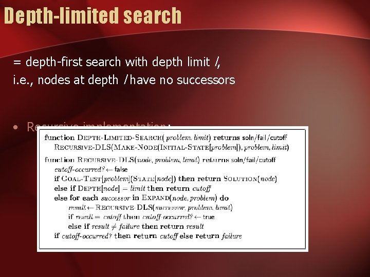
Depth-limited search = depth-first search with depth limit l, i. e. , nodes at depth l have no successors • Recursive implementation:

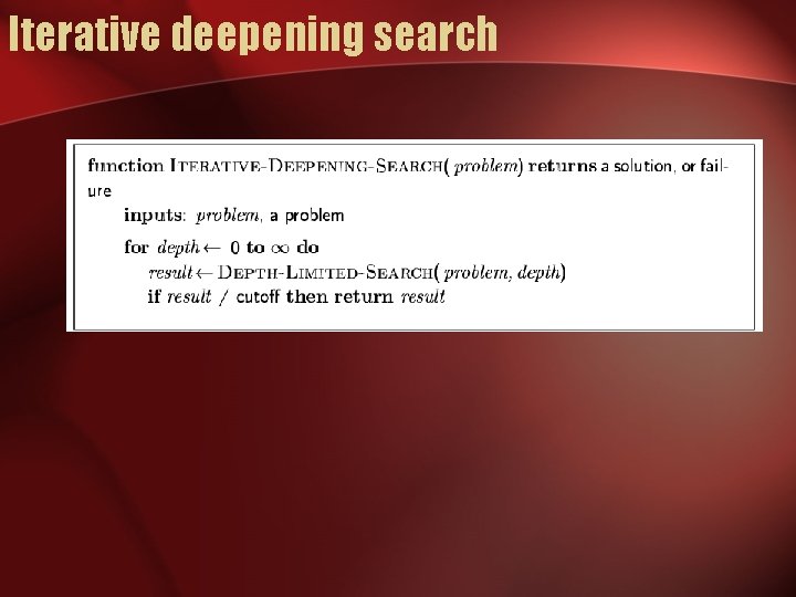
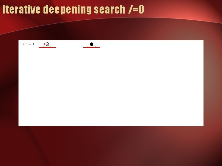
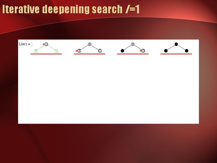
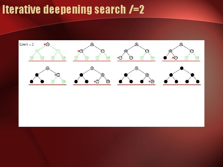
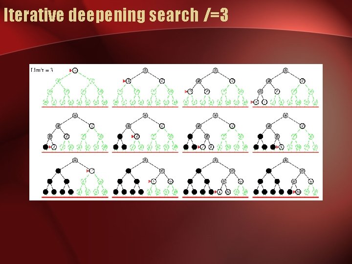
Iterative deepening search

Iterative deepening search l =0

Iterative deepening search l =1

Iterative deepening search l =2

Iterative deepening search l =3

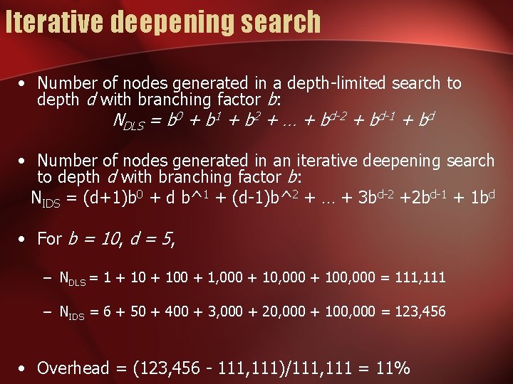
Iterative deepening search • Number of nodes generated in a depth-limited search to depth d with branching factor b: NDLS = b 0 + b 1 + b 2 + … + bd-2 + bd-1 + bd • Number of nodes generated in an iterative deepening search to depth d with branching factor b: NIDS = (d+1)b 0 + d b^1 + (d-1)b^2 + … + 3 bd-2 +2 bd-1 + 1 bd • For b = 10, d = 5, – NDLS = 1 + 100 + 1, 000 + 100, 000 = 111, 111 – NIDS = 6 + 50 + 400 + 3, 000 + 20, 000 + 100, 000 = 123, 456 • Overhead = (123, 456 - 111, 111)/111, 111 = 11%

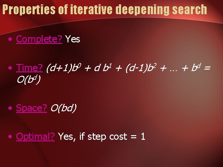
Properties of iterative deepening search • Complete? Yes • Time? (d+1)b 0 + d b 1 + (d-1)b 2 + … + bd = O(bd) • Space? O(bd) • Optimal? Yes, if step cost = 1

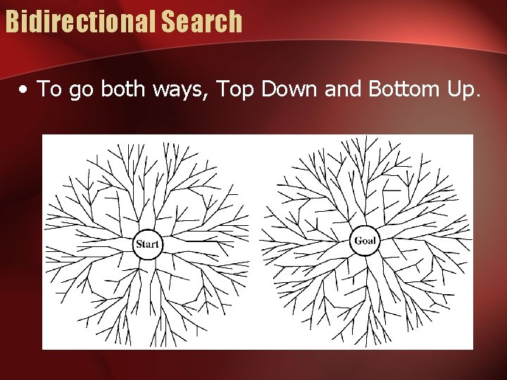
Bidirectional Search • To go both ways, Top Down and Bottom Up.

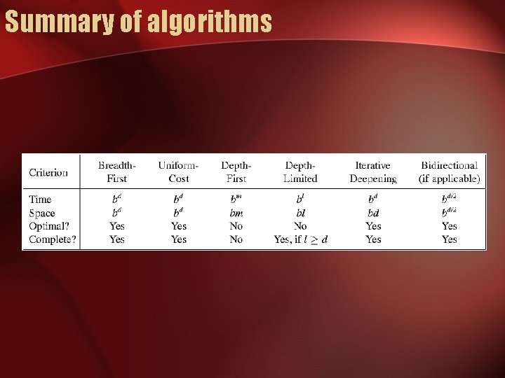
Summary of algorithms

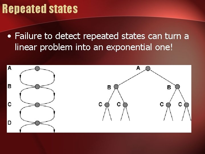
Repeated states • Failure to detect repeated states can turn a linear problem into an exponential one!

Repeated states • Do not return to the state you just came from. • Do not create paths with cycles in them. • Do not generate any state that was ever generated before. – Hashing

Constraint Satisfaction Search • Constraint Satisfaction Search: a special kind of search problem. States: a set of variables Goal Test: a set of constraints that the values must obey. – Absolute/Preferred Constraints – Variable Domain – Back Tracking – Forward Checking / Arc Consistency

Summary • Problem formulation usually requires abstracting away realworld details to define a state space that can feasibly be explored • Variety of uninformed search strategies – – – Breadth First Search Depth First Search Uniform Cost Search (Best First Search) Depth Limited Search Iterative Deepening Bidirectional Search

Ex. ERCi. SES! • Exercises 3. 9: – Implement the missionaries and cannibals problem and use an a search method to find the shortest path. Is it useful to keep track of repeated cases? • Exercise 3. X: – Assume a set of N chain links with some a priory connections. Assuming an operator that connects/disconnects two links. Formulate a search problem and find the optimal solution from a given initial state to a given goal state. • • Due: Esfand, 15 th Language: C++ / Java Mail To: n_ghanbari@ce. sharif. edu Subject: AIEX-CANNIBALS, AIEX-CHAINS