AN INDEPTH ANALYSIS OF LOGARITHMIC DATA TRANSFORMATION AND

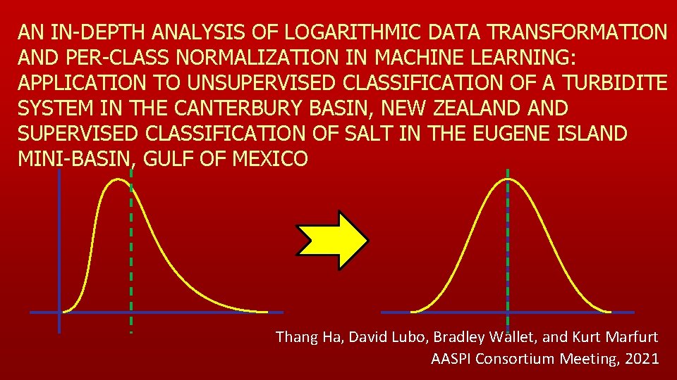
AN IN-DEPTH ANALYSIS OF LOGARITHMIC DATA TRANSFORMATION AND PER-CLASS NORMALIZATION IN MACHINE LEARNING: APPLICATION TO UNSUPERVISED CLASSIFICATION OF A TURBIDITE SYSTEM IN THE CANTERBURY BASIN, NEW ZEALAND SUPERVISED CLASSIFICATION OF SALT IN THE EUGENE ISLAND MINI-BASIN, GULF OF MEXICO Thang Ha, David Lubo, Bradley Wallet, and Kurt Marfurt AASPI Consortium Meeting, 2021

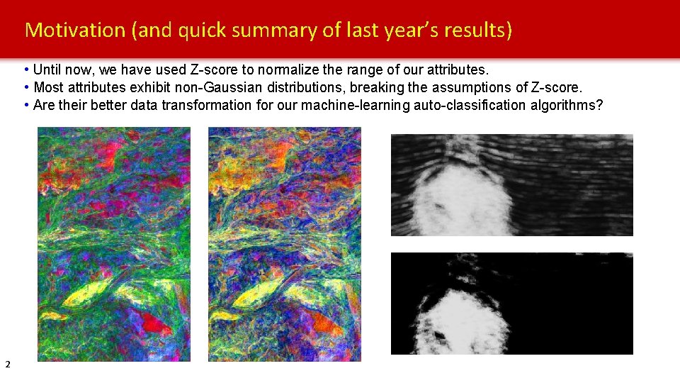
Motivation (and quick summary of last year’s results) • Until now, we have used Z-score to normalize the range of our attributes. • Most attributes exhibit non-Gaussian distributions, breaking the assumptions of Z-score. • Are their better data transformation for our machine-learning auto-classification algorithms? 2

Outline • Motivation • Case Study 1: Turbidite – New Zealand o PCA results o ICA results o SOM results o GTM results • Case Study 2: Salt – Gulf of Mexico o Bulk vs per-class normalization o PNN Prediction results o PNN Probability results • Explanation: why is A better than B? • Conclusions 3

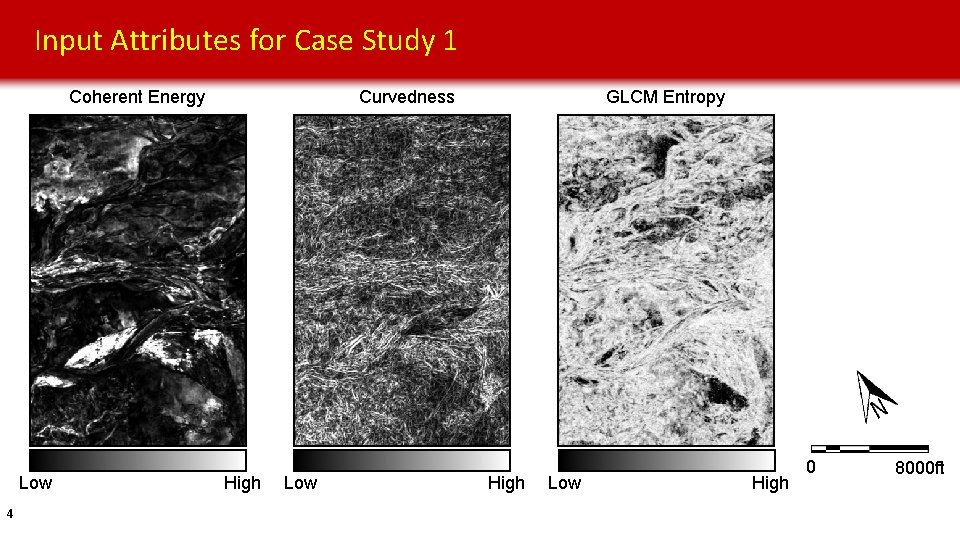
Input Attributes for Case Study 1 Curvedness Coherent Energy Low 4 High Low GLCM Entropy High Low High 0 8000 ft

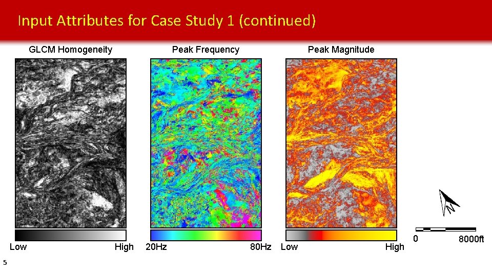
Input Attributes for Case Study 1 (continued) Peak Frequency GLCM Homogeneity Low 5 High 20 Hz Peak Magnitude 80 Hz Low High 0 8000 ft

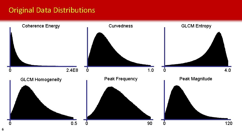
Original Data Distributions Coherence Energy 0 Curvedness 2. 4 E 8 0 6 1. 0 0 Peak Frequency GLCM Homogeneity 0 GLCM Entropy 0. 5 0 4. 0 Peak Magnitude 90 0 120

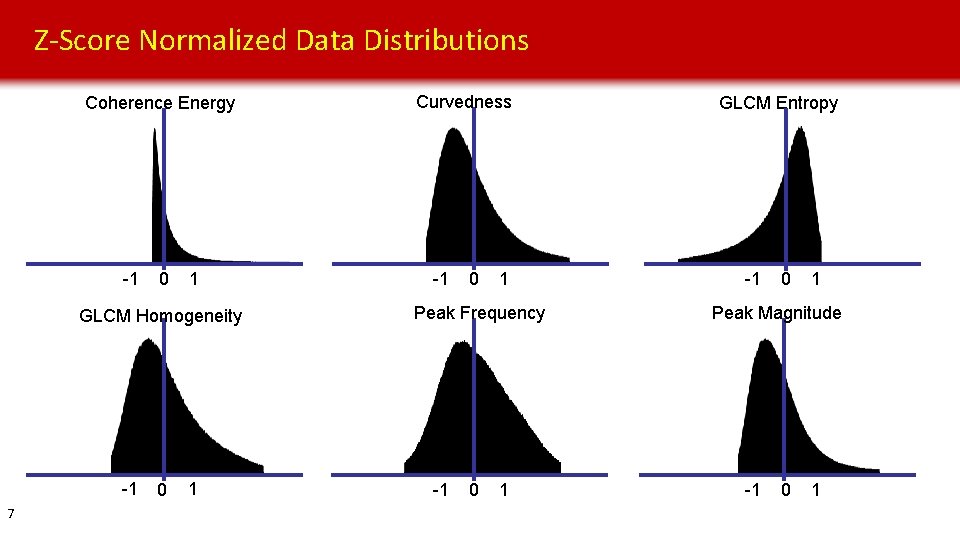
Z-Score Normalized Data Distributions Coherence Energy -1 0 1 GLCM Homogeneity -1 7 0 1 Curvedness -1 0 1 Peak Frequency -1 0 1 GLCM Entropy -1 0 1 Peak Magnitude -1 0 1

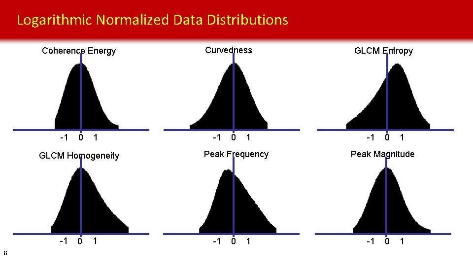
Logarithmic Normalized Data Distributions Coherence Energy -1 0 1 GLCM Homogeneity -1 8 0 1 Curvedness -1 0 1 Peak Frequency -1 0 1 GLCM Entropy -1 0 1 Peak Magnitude -1 0 1

Outline • Motivation • Case Study 1: Turbidite – New Zealand o PCA results o ICA results o SOM results o GTM results • Case Study 2: Salt – Gulf of Mexico o Bulk vs per-class normalization o PNN Prediction results o PNN Probability results • Explanation: why is A better than B? • Conclusions 9

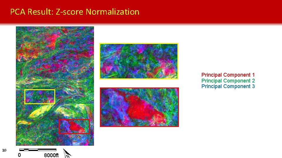
PCA Result: Z-score Normalization Principal Component 1 Principal Component 2 Principal Component 3 10 0 8000 ft

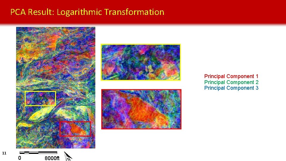
PCA Result: Logarithmic Transformation Principal Component 1 Principal Component 2 Principal Component 3 11 0 8000 ft

Outline • Motivation • Case Study 1: Turbidite – New Zealand o PCA results o ICA results o SOM results o GTM results • Case Study 2: Salt – Gulf of Mexico o Bulk vs per-class normalization o PNN Prediction results o PNN Probability results • Explanation: why is A better than B? • Conclusions 12

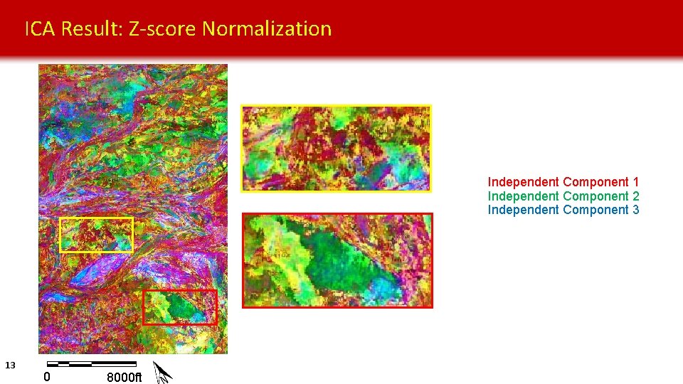
ICA Result: Z-score Normalization Independent Component 1 Independent Component 2 Independent Component 3 13 0 8000 ft

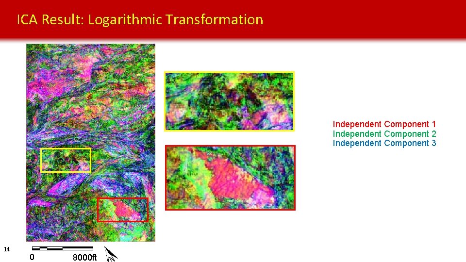
ICA Result: Logarithmic Transformation Independent Component 1 Independent Component 2 Independent Component 3 14 0 8000 ft

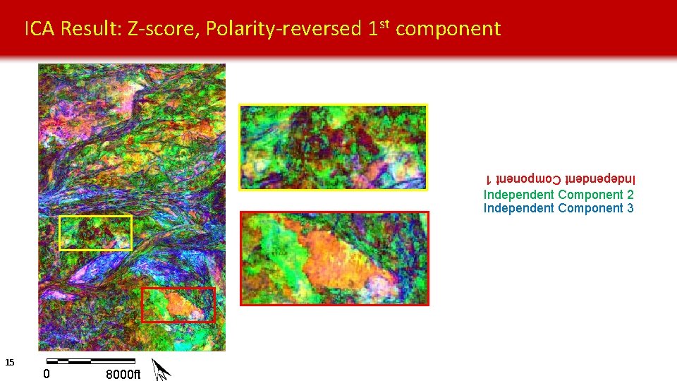
ICA Result: Z-score, Polarity-reversed 1 st component Independent Component 1 Independent Component 2 Independent Component 3 15 0 8000 ft

Outline • Motivation • Case Study 1: Turbidite – New Zealand o PCA results o ICA results o SOM results o GTM results • Case Study 2: Salt – Gulf of Mexico o Bulk vs per-class normalization o PNN Prediction results o PNN Probability results • Explanation: why is A better than B? • Conclusions 16

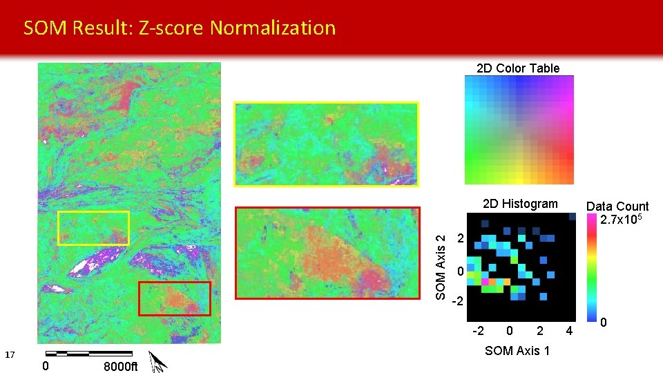
SOM Result: Z-score Normalization 2 D Color Table SOM Axis 2 2 D Histogram 2 0 -2 -2 17 0 2 SOM Axis 1 0 8000 ft Data Count 2. 7 x 105 4 0

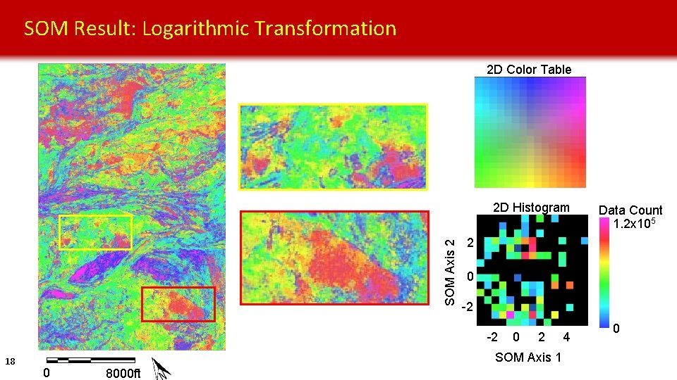
SOM Result: Logarithmic Transformation 2 D Color Table SOM Axis 2 2 D Histogram 2 0 -2 -2 18 0 2 SOM Axis 1 0 8000 ft Data Count 1. 2 x 105 4 0

Outline • Motivation • Case Study 1: Turbidite – New Zealand o PCA results o ICA results o SOM results o GTM results • Case Study 2: Salt – Gulf of Mexico o Bulk vs per-class normalization o PNN Prediction results o PNN Probability results • Explanation: why is A better than B? • Conclusions 19

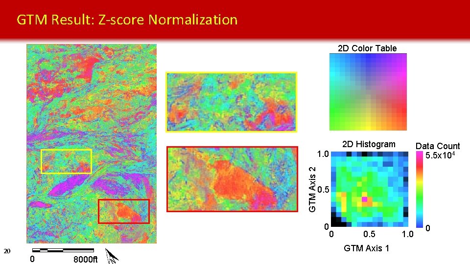
GTM Result: Z-score Normalization 2 D Color Table 2 D Histogram Data Count 5. 5 x 104 GTM Axis 2 1. 0 0. 5 0 20 0 0. 5 GTM Axis 1 0 8000 ft 1. 0 0

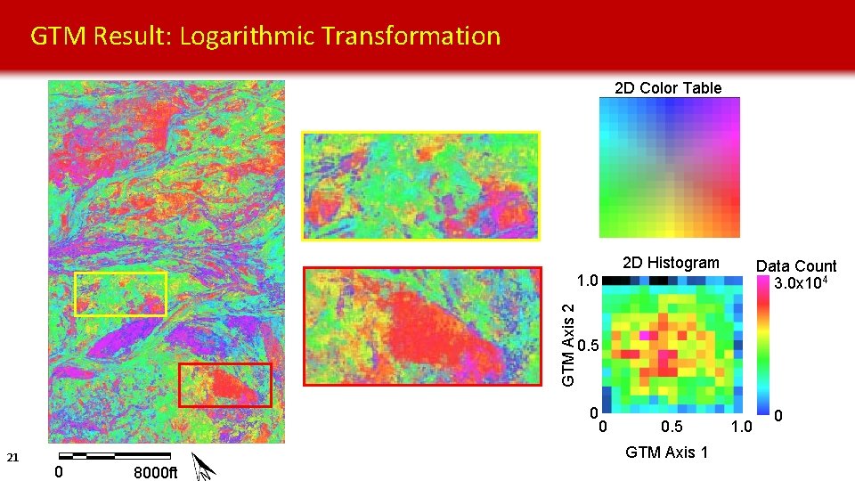
GTM Result: Logarithmic Transformation 2 D Color Table 2 D Histogram Data Count 3. 0 x 104 GTM Axis 2 1. 0 0. 5 0 21 0 0. 5 GTM Axis 1 0 8000 ft 1. 0 0

Outline • Motivation • Case Study 1: Turbidite – New Zealand o PCA results o ICA results o SOM results o GTM results • Case Study 2: Salt – Gulf of Mexico o Bulk vs per-class normalization o PNN Prediction results o PNN Probability results • Explanation: why is A better than B? • Conclusions 22

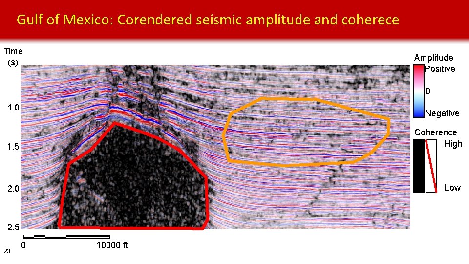
Gulf of Mexico: Corendered seismic amplitude and coherece Time (s) Amplitude Positive 0 1. 0 Negative 1. 5 Coherence High 2. 0 Low 2. 5 23 0 10000 ft

Outline • Motivation • Case Study 1: Turbidite – New Zealand o PCA results o ICA results o SOM results o GTM results • Case Study 2: Salt – Gulf of Mexico o Bulk vs per-class normalization o PNN Prediction results o PNN Probability results • Explanation: why is A better than B? • Conclusions 24

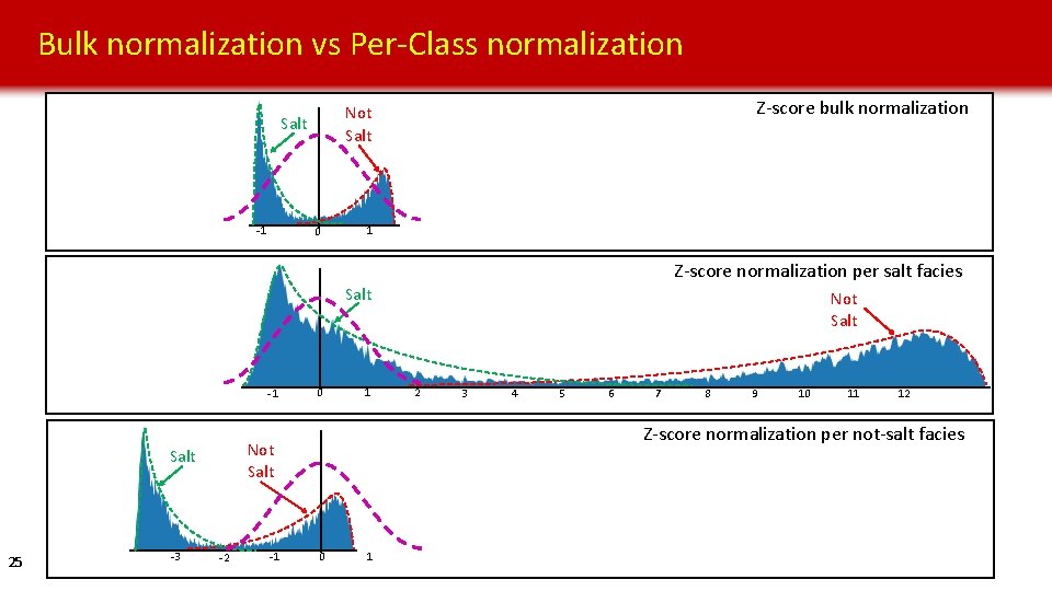
Bulk normalization vs Per-Class normalization Salt -1 Z-score bulk normalization Not Salt 0 1 Z-score normalization per salt facies Salt -1 -3 1 -2 -1 2 3 4 5 6 7 8 9 10 11 12 Z-score normalization per not-salt facies Not Salt 25 0 Not Salt 0 1

Outline • Motivation • Case Study 1: Turbidite – New Zealand o PCA results o ICA results o SOM results o GTM results • Case Study 2: Salt – Gulf of Mexico o Bulk vs per-class normalization o PNN Prediction results o PNN Probability results • Explanation: why is A better than B? • Conclusions 26

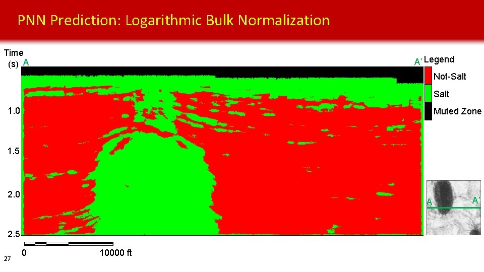
PNN Prediction: Logarithmic Bulk Normalization Time (s) A A’ Legend Not-Salt 1. 0 Muted Zone 1. 5 2. 0 A 2. 5 27 0 10000 ft A’

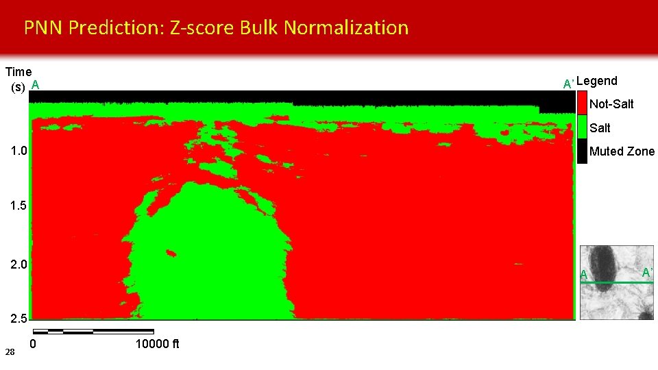
PNN Prediction: Z-score Bulk Normalization Time (s) A A’ Legend Not-Salt 1. 0 Muted Zone 1. 5 2. 0 A 2. 5 28 0 10000 ft A’

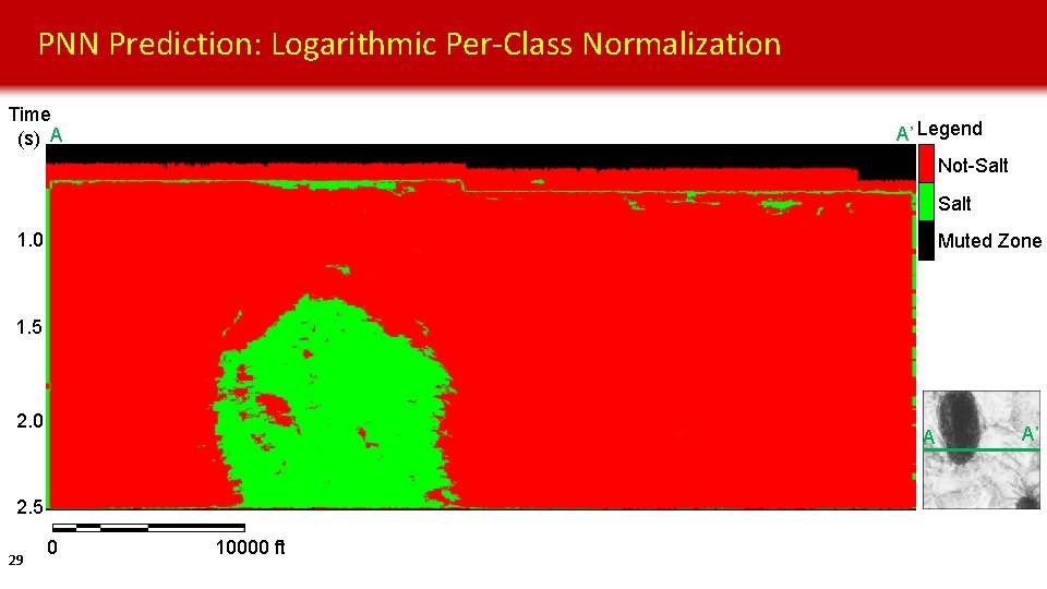
PNN Prediction: Logarithmic Per-Class Normalization Time (s) A A’ Legend Not-Salt 1. 0 Muted Zone 1. 5 2. 0 A 2. 5 29 0 10000 ft A’

PNN Prediction: Z-score Per-Class Normalization Time (s) A A’ Legend Not-Salt 1. 0 Muted Zone 1. 5 2. 0 A 2. 5 30 0 10000 ft A’

Outline • Motivation • Case Study 1: Turbidite – New Zealand o PCA results o ICA results o SOM results o GTM results • Case Study 2: Salt – Gulf of Mexico o Bulk vs per-class normalization o PNN Prediction results o PNN Probability results • Explanation: why is A better than B? • Conclusions 31

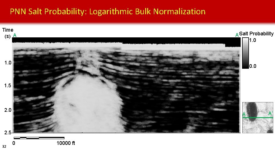
PNN Salt Probability: Logarithmic Bulk Normalization Time (s) A A’Salt Probability 1. 0 0. 0 1. 5 2. 0 A 2. 5 32 0 10000 ft A’

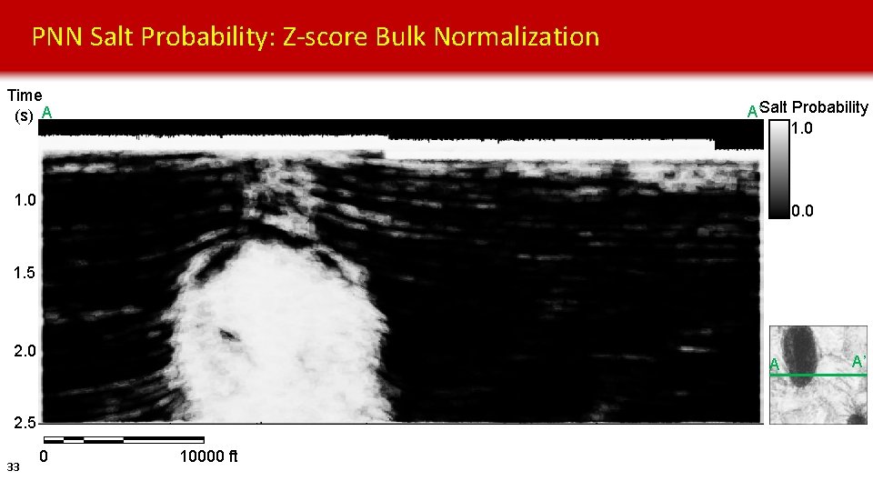
PNN Salt Probability: Z-score Bulk Normalization Time (s) A A’Salt Probability 1. 0 0. 0 1. 5 2. 0 A 2. 5 33 0 10000 ft A’

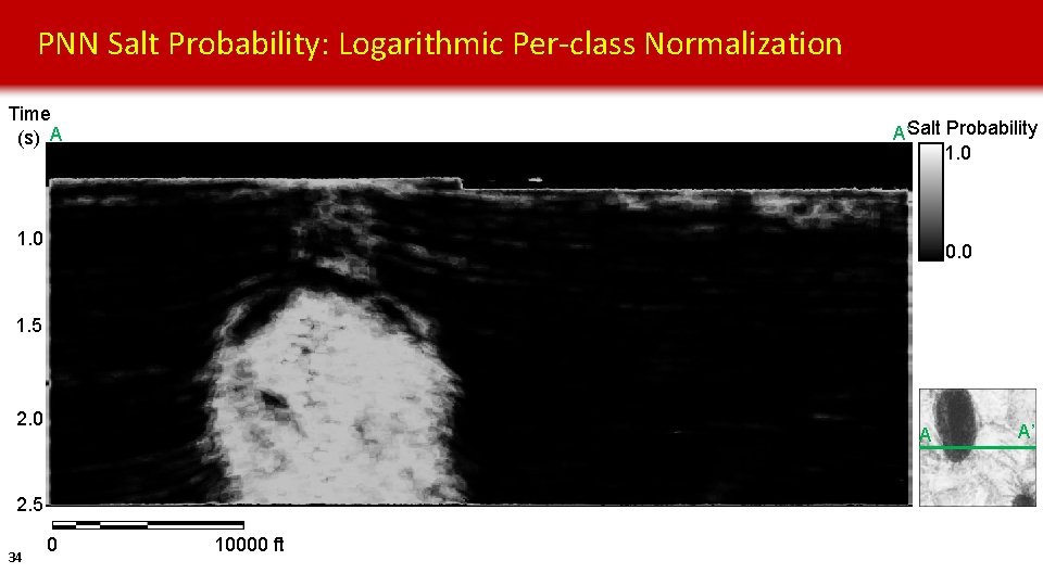
PNN Salt Probability: Logarithmic Per-class Normalization Time (s) A A’Salt Probability 1. 0 0. 0 1. 5 2. 0 A 2. 5 34 0 10000 ft A’

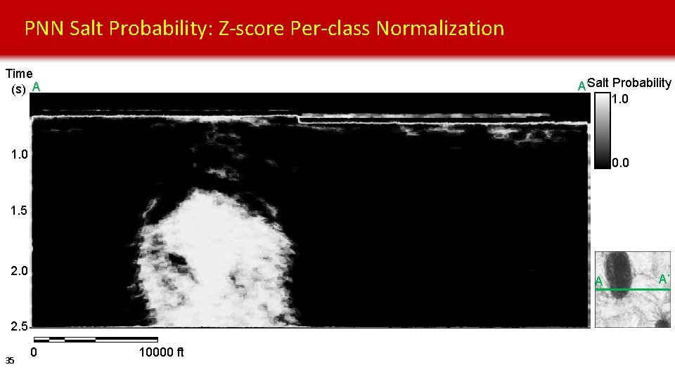
PNN Salt Probability: Z-score Per-class Normalization Time (s) A A’Salt Probability 1. 0 0. 0 1. 5 2. 0 A 2. 5 35 0 10000 ft A’

Outline • Motivation • Case Study 1: Turbidite – New Zealand o PCA results o ICA results o SOM results o GTM results • Case Study 2: Salt – Gulf of Mexico o Bulk vs per-class normalization o PNN Prediction results o PNN Probability results • Explanation: why is A better than B? • Conclusions 36

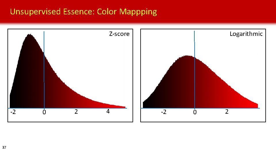
Unsupervised Essence: Color Mappping Logarithmic Z-score -2 37 0 2 4 -2 0 2

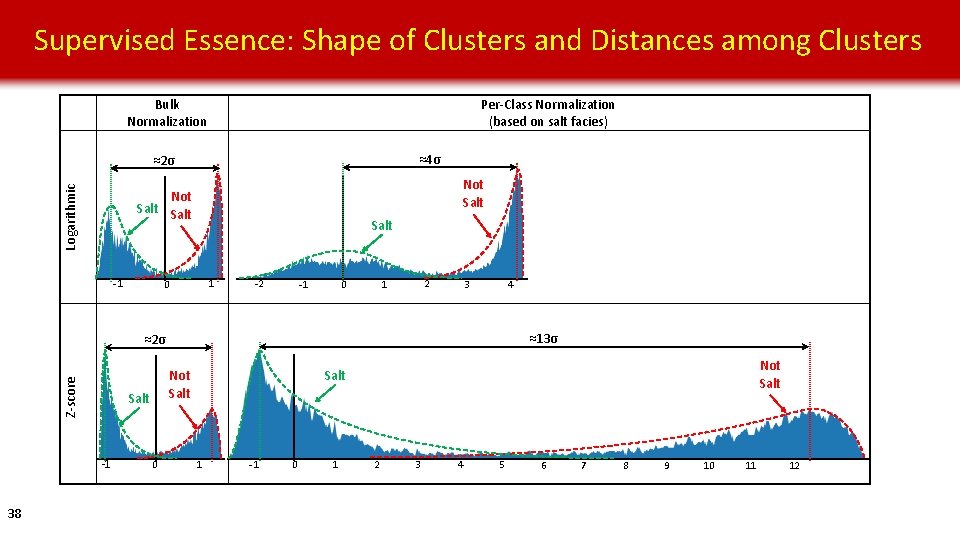
Supervised Essence: Shape of Clusters and Distances among Clusters Per-Class Normalization (based on salt facies) Bulk Normalization ≈4σ Logarithmic ≈2σ Not Salt -1 Salt 1 0 -2 2 1 0 -1 3 4 ≈13σ Z-score ≈2σ Salt -1 38 Not Salt 0 Not Salt 1 -1 0 1 2 3 4 5 6 7 8 9 10 11 12

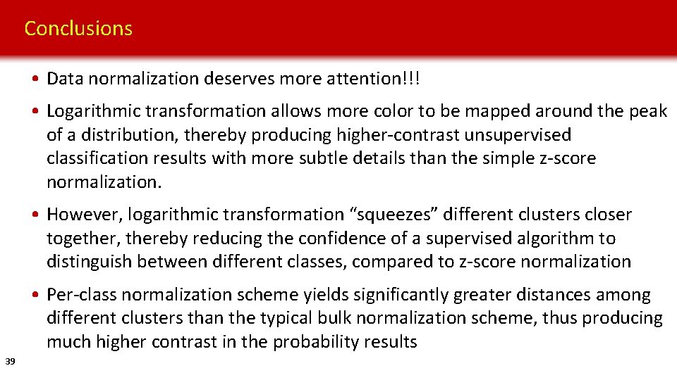
Conclusions • Data normalization deserves more attention!!! • Logarithmic transformation allows more color to be mapped around the peak of a distribution, thereby producing higher-contrast unsupervised classification results with more subtle details than the simple z-score normalization. • However, logarithmic transformation “squeezes” different clusters closer together, thereby reducing the confidence of a supervised algorithm to distinguish between different classes, compared to z-score normalization • Per-class normalization scheme yields significantly greater distances among different clusters than the typical bulk normalization scheme, thus producing much higher contrast in the probability results 39

BACKUP SLIDES

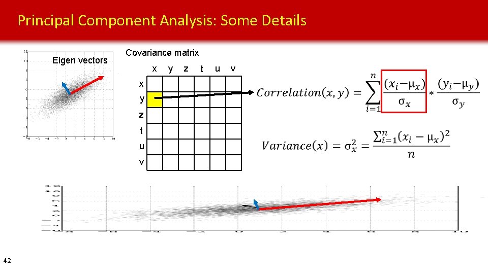
Principal Component Analysis: Some Details Eigen vectors Covariance matrix x x y z t u v 42 y z t u v

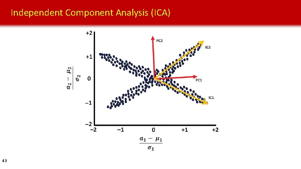
Independent Component Analysis (ICA) 43

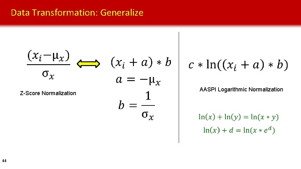
Data Transformation: Generalize Z-Score Normalization 44 AASPI Logarithmic Normalization

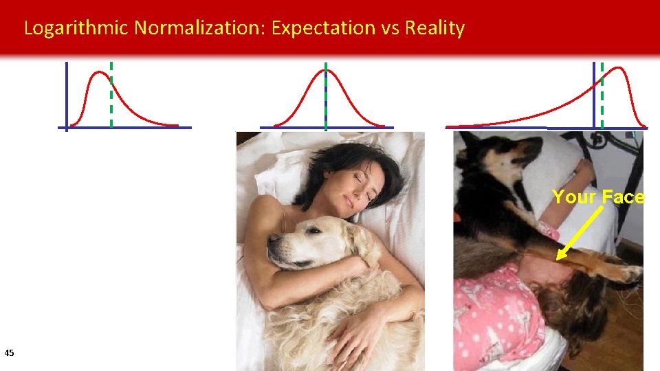
Logarithmic Normalization: Expectation vs Reality Your Face 45

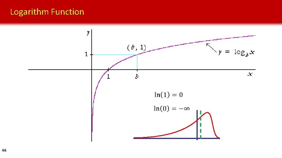
Logarithm Function 46

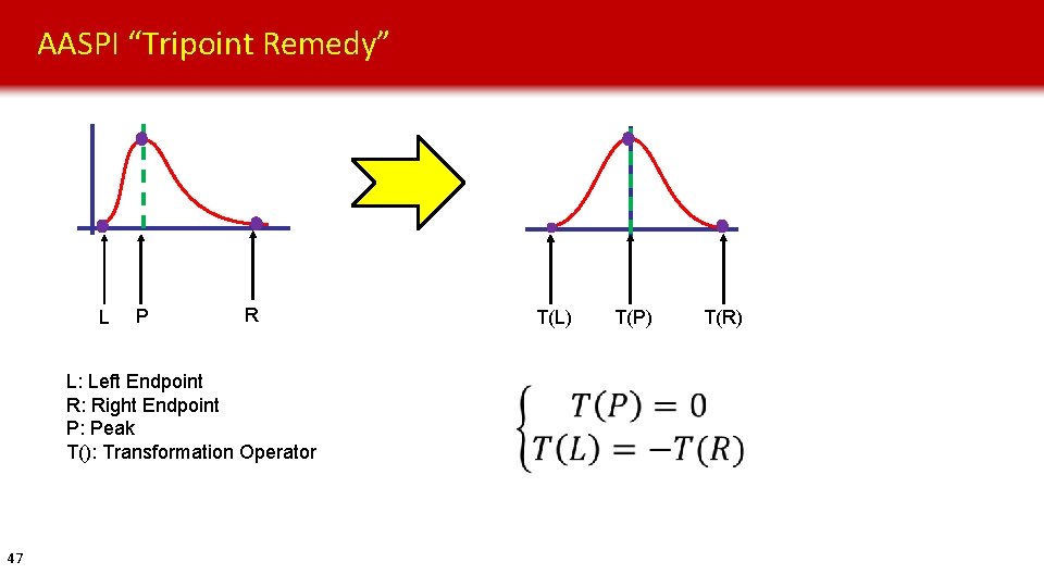
AASPI “Tripoint Remedy” L P R L: Left Endpoint R: Right Endpoint P: Peak T(): Transformation Operator 47 T(L) T(P) T(R)

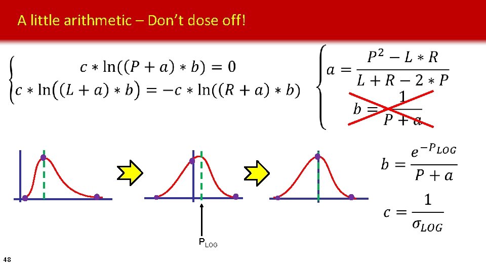
A little arithmetic – Don’t dose off! PLOG 48

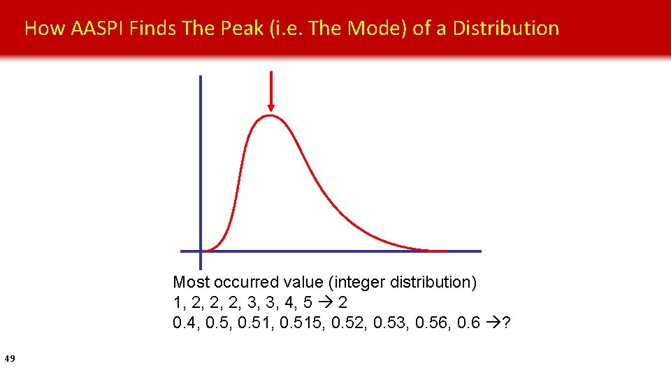
How AASPI Finds The Peak (i. e. The Mode) of a Distribution Most occurred value (integer distribution) 1, 2, 2, 2, 3, 3, 4, 5 2 0. 4, 0. 51, 0. 515, 0. 52, 0. 53, 0. 56, 0. 6 ? 49

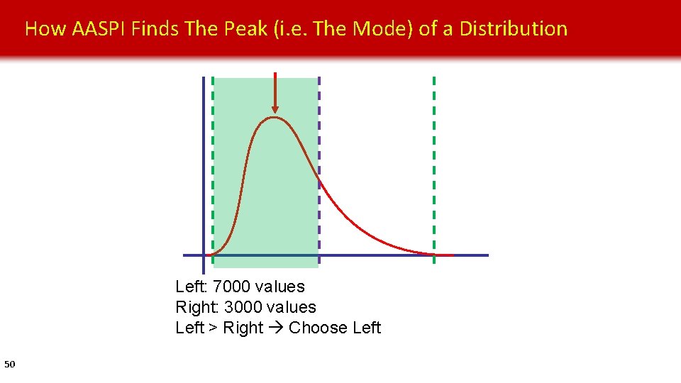
How AASPI Finds The Peak (i. e. The Mode) of a Distribution Left: 7000 values Right: 3000 values Left > Right Choose Left 50

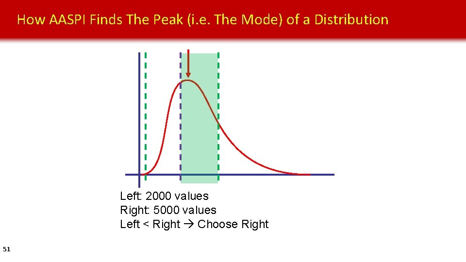
How AASPI Finds The Peak (i. e. The Mode) of a Distribution Left: 2000 values Right: 5000 values Left < Right Choose Right 51

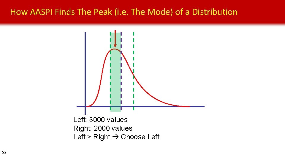
How AASPI Finds The Peak (i. e. The Mode) of a Distribution Left: 3000 values Right: 2000 values Left > Right Choose Left 52

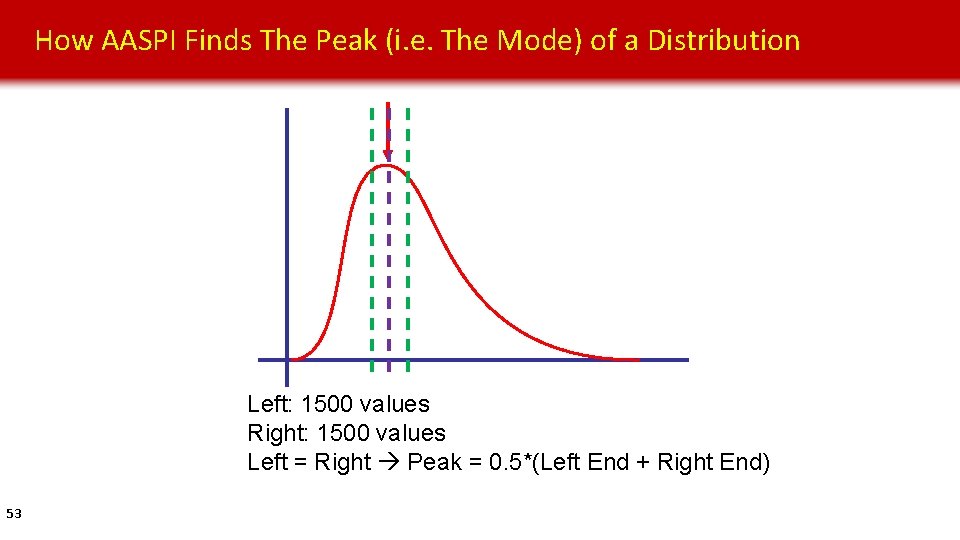
How AASPI Finds The Peak (i. e. The Mode) of a Distribution Left: 1500 values Right: 1500 values Left = Right Peak = 0. 5*(Left End + Right End) 53

Log-Normal Coherent Energy: Shift = 0, Scale =1 Principle Component 1 Coherent Energy 0 0 -1. 0 54 0. 0 1. 5 Low High 8000 ft

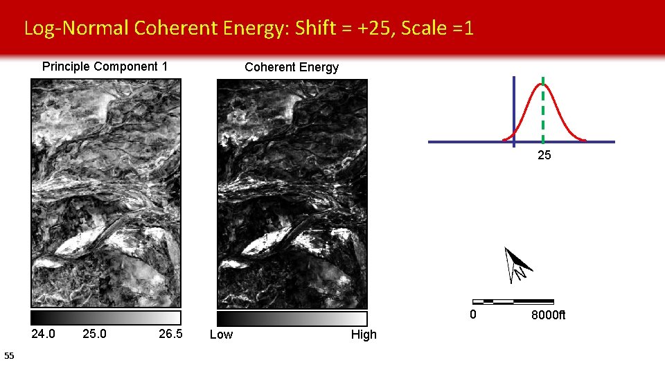
Log-Normal Coherent Energy: Shift = +25, Scale =1 Principle Component 1 Coherent Energy 25 0 24. 0 55 25. 0 26. 5 Low High 8000 ft

Log-Normal Coherent Energy: Shift = 0, Scale =1 Principle Component 1 Coherent Energy 0 0 -1. 0 56 0. 0 1. 5 Low High 8000 ft

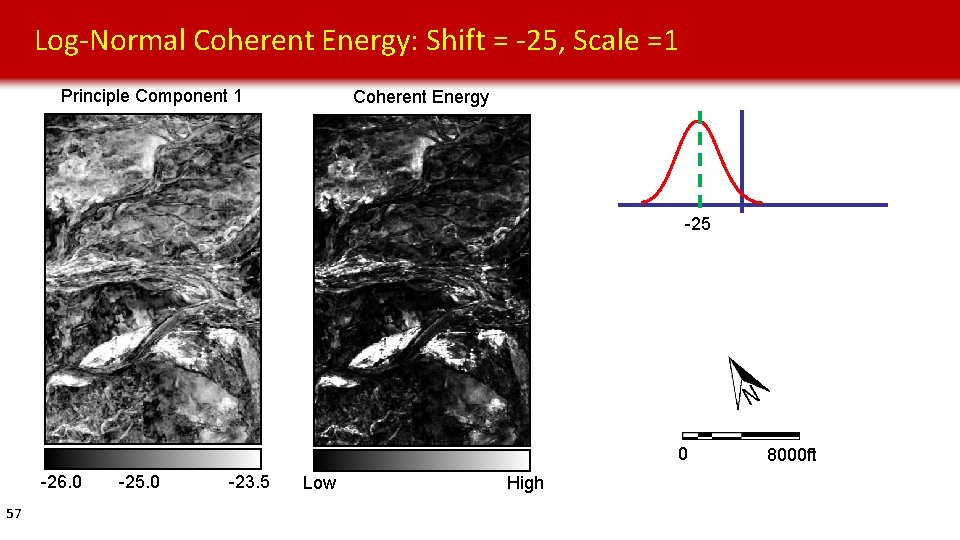
Log-Normal Coherent Energy: Shift = -25, Scale =1 Principle Component 1 Coherent Energy -25 0 -26. 0 57 -25. 0 -23. 5 Low High 8000 ft

Log-Normal Coherent Energy: Shift = 0, Scale =1 Principle Component 1 Coherent Energy 0 0 -1. 0 58 0. 0 1. 5 Low High 8000 ft

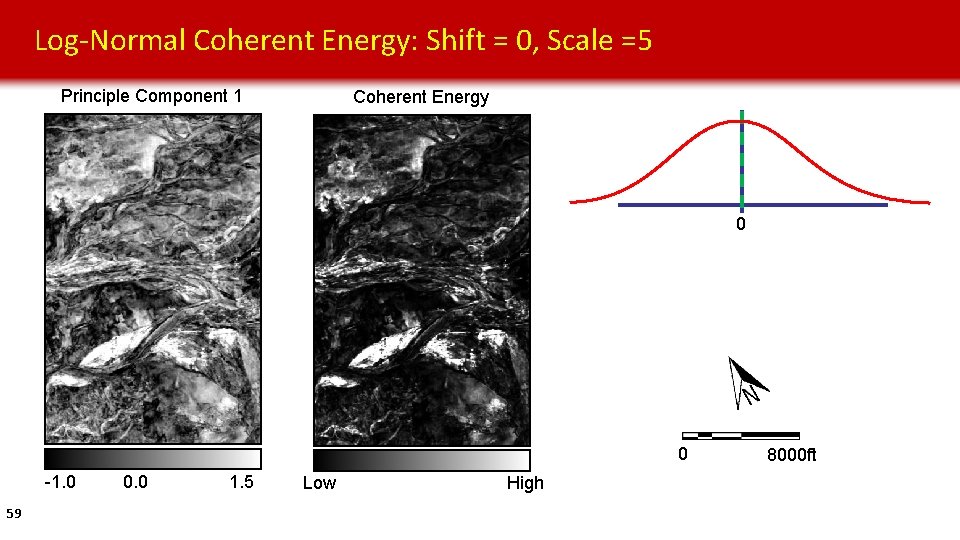
Log-Normal Coherent Energy: Shift = 0, Scale =5 Principle Component 1 Coherent Energy 0 0 -1. 0 59 0. 0 1. 5 Low High 8000 ft

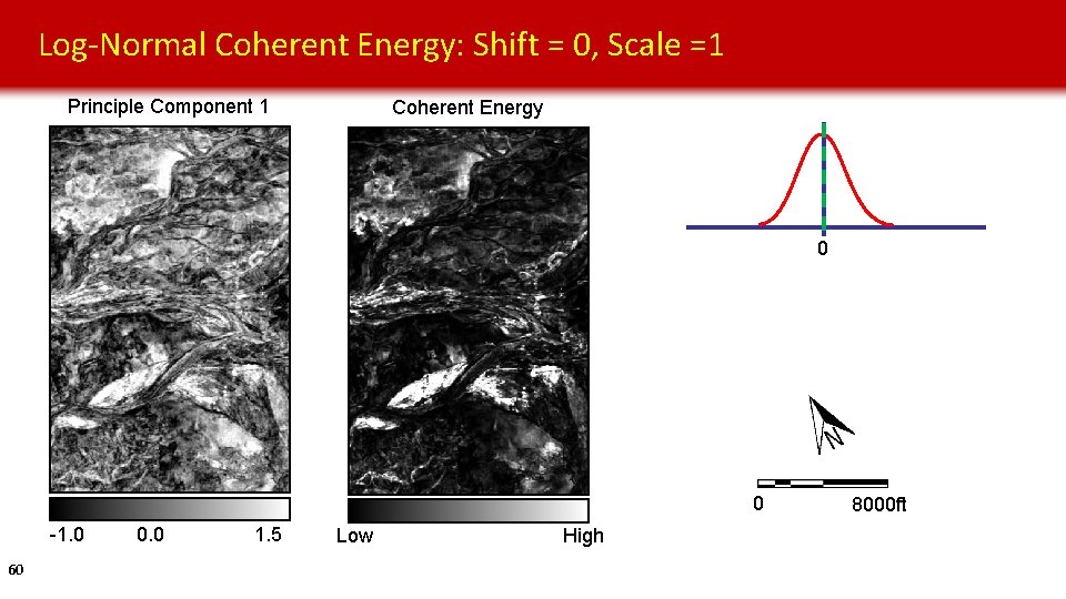
Log-Normal Coherent Energy: Shift = 0, Scale =1 Principle Component 1 Coherent Energy 0 0 -1. 0 60 0. 0 1. 5 Low High 8000 ft

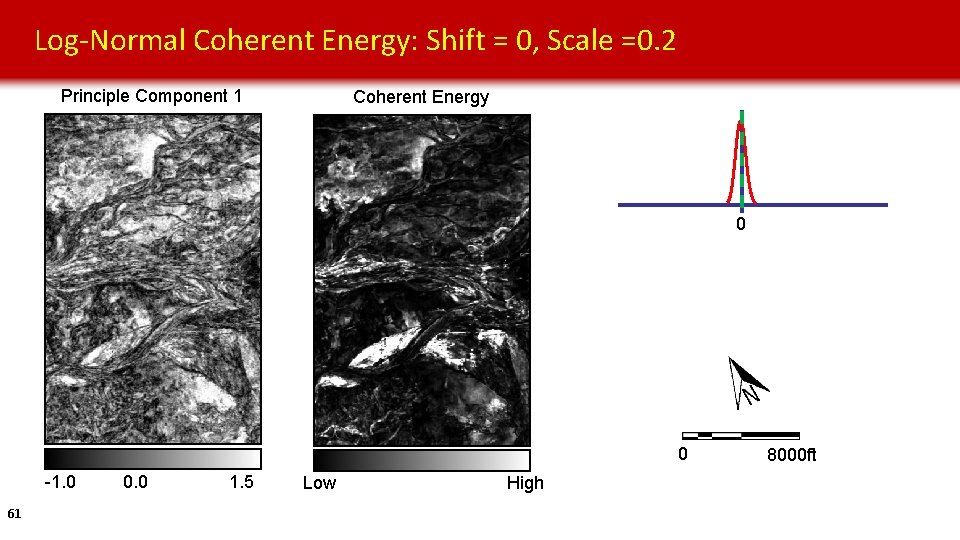
Log-Normal Coherent Energy: Shift = 0, Scale =0. 2 Principle Component 1 Coherent Energy 0 0 -1. 0 61 0. 0 1. 5 Low High 8000 ft

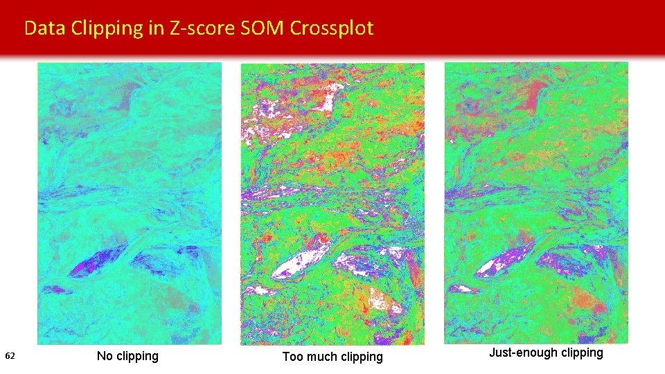
Data Clipping in Z-score SOM Crossplot 62 No clipping Too much clipping Just-enough clipping