An Improved Algorithm for the Rectangle Enclosure Problem

An Improved Algorithm for the Rectangle Enclosure Problem Anatoli Uchitel From an article By D. T. Lee and F. P. Preparata (March 8, 1981)

Introduction w This essay gives an algorithm for solving the Rectangle Enclosure problem in time and O(n) space w n is the number of rectangles and q is the number of the required rectangle pairs

Topics of Presentation w Introduction w Rectangle Enclosure and Dominance w A Two-Dimensional Subproblem w Time and Space Analysis

Introduction What is the Rectangle Enclosure problem ? Given a set of n rectangles in the plane, with sides parallel to the coordinate axes , find all q pairs of rectangles such that one rectangle of the pair encloses the other w The suggested solution achieves time using O(n) space w

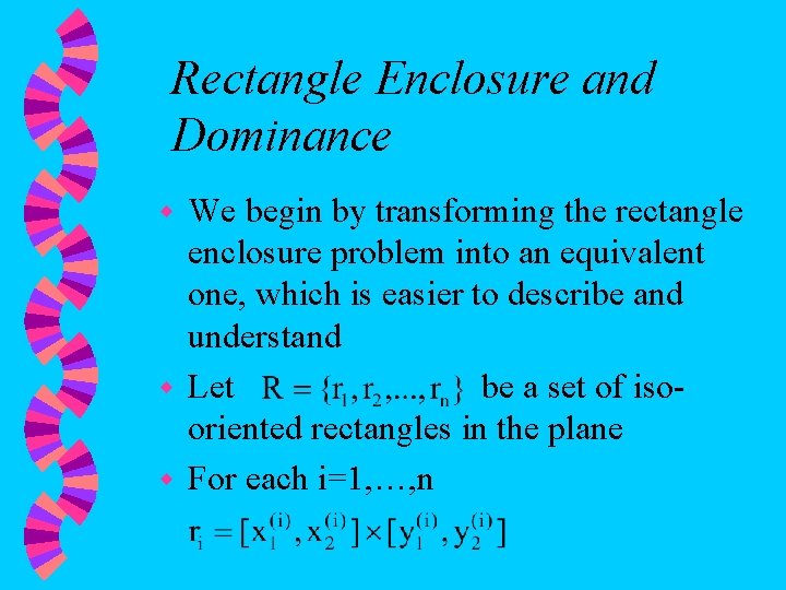
Rectangle Enclosure and Dominance We begin by transforming the rectangle enclosure problem into an equivalent one, which is easier to describe and understand w Let be a set of isooriented rectangles in the plane w For each i=1, …, n w

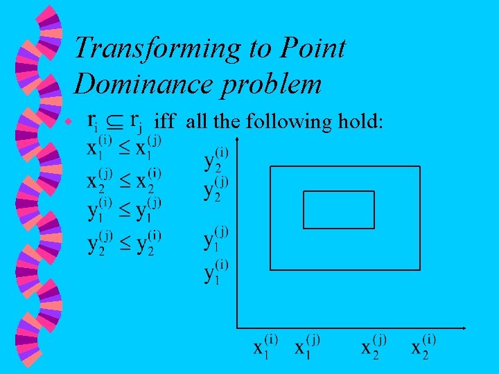
Transforming to Point Dominance problem w iff all the following hold:

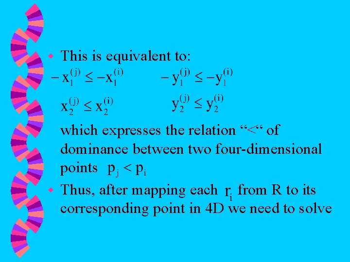
w This is equivalent to: which expresses the relation “<“ of dominance between two four-dimensional points w Thus, after mapping each from R to its corresponding point in 4 D we need to solve

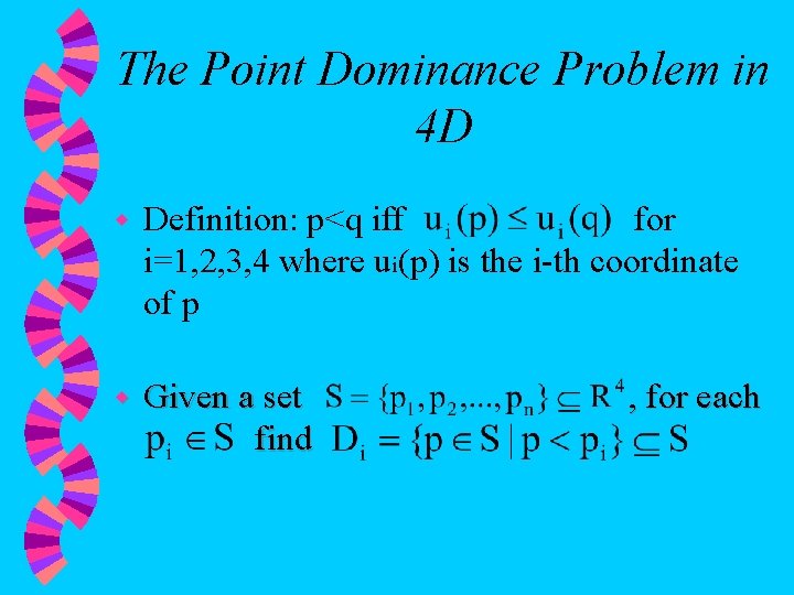
The Point Dominance Problem in 4 D w Definition: p<q iff for i=1, 2, 3, 4 where ui(p) is the i-th coordinate of p w Given a set find , for each

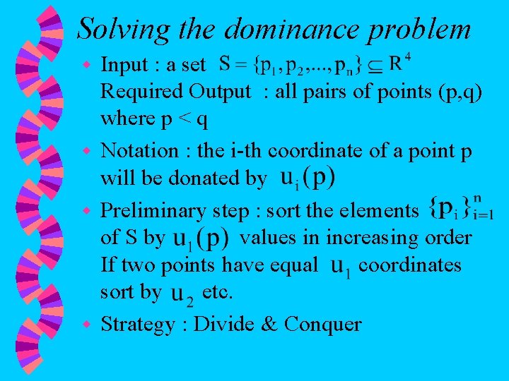
Solving the dominance problem Input : a set Required Output : all pairs of points (p, q) where p < q w Notation : the i-th coordinate of a point p will be donated by w Preliminary step : sort the elements of S by values in increasing order If two points have equal coordinates sort by etc. w Strategy : Divide & Conquer w

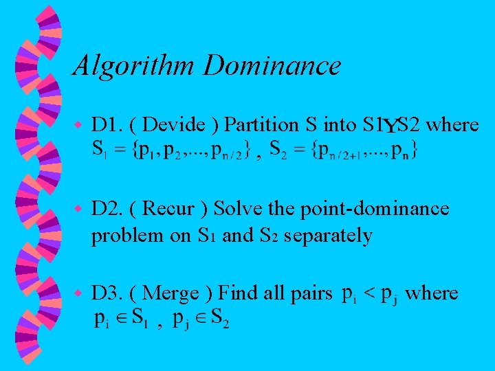
Algorithm Dominance w D 1. ( Devide ) Partition S into S 1 S 2 where , w D 2. ( Recur ) Solve the point-dominance problem on S 1 and S 2 separately w D 3. ( Merge ) Find all pairs , where

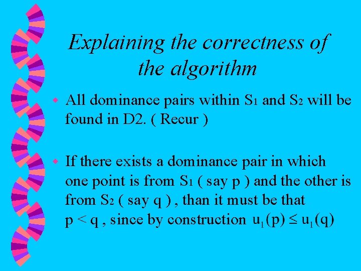
Explaining the correctness of the algorithm w All dominance pairs within S 1 and S 2 will be found in D 2. ( Recur ) w If there exists a dominance pair in which one point is from S 1 ( say p ) and the other is from S 2 ( say q ) , than it must be that p < q , since by construction

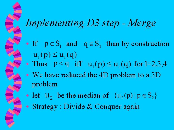
Implementing D 3 step - Merge w If and than by construction Thus iff for l=2, 3, 4 w We have reduced the 4 D problem to a 3 D problem w let be the median of w Strategy : Divide & Conquer again w

Algorithm Merge w M 1. ( devide ) Partition S 1 into S 11 S 12 and S 2 into S 21 S 22 where S 12 = S 1 -S 11 S 22 = S 2 -S 21 M 2. ( Recur ) Solve the merge problem on the set pairs (S 11, S 21) and (S 12, S 22) w M 3. (Combine) Find all pairs pi<pj such that and w

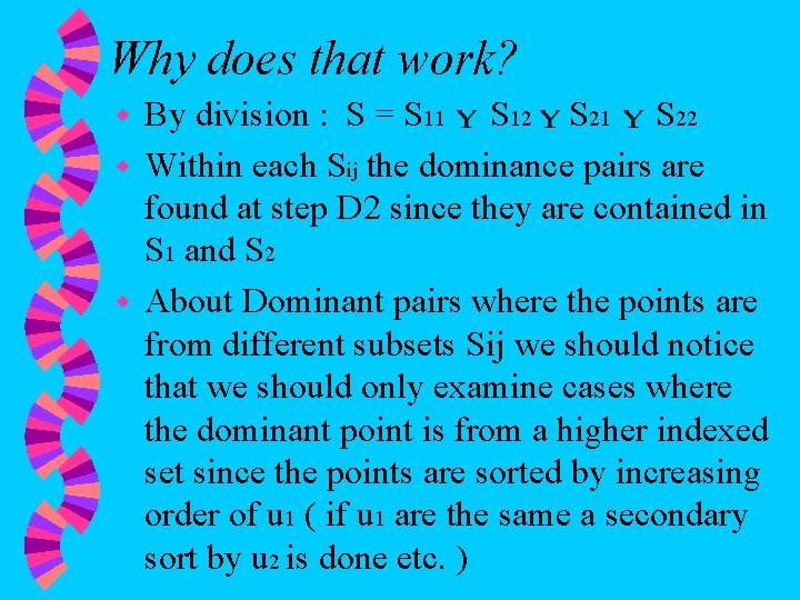
Why does that work? By division : S = S 11 S 12 S 21 S 22 w Within each Sij the dominance pairs are found at step D 2 since they are contained in S 1 and S 2 w About Dominant pairs where the points are from different subsets Sij we should notice that we should only examine cases where the dominant point is from a higher indexed set since the points are sorted by increasing order of u 1 ( if u 1 are the same a secondary sort by u 2 is done etc. ) w

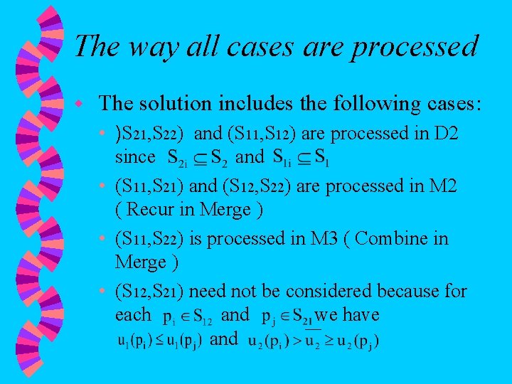
The way all cases are processed w The solution includes the following cases: • )S 21, S 22) and (S 11, S 12) are processed in D 2 since and • (S 11, S 21) and (S 12, S 22) are processed in M 2 ( Recur in Merge ) • (S 11, S 22) is processed in M 3 ( Combine in Merge ) • (S 12, S 21) need not be considered because for each and we have and

Implementation of the Combine w The key operation of the entire task is therefore the implementation of step M 3 ( the combine ) w Again we reduce the dimension of the problem, since the Combine step is a 2 D merge problem ( in u 3 and u 4 )

A Two-Dimensional Subproblem Initial preprocessing : Construct a quadruply threaded list ( QTL ) with bidirectional links, for S. w for each p in S there is a node containing all the coordinate values and 8 pointers NEXTi, PREVi for i=1, 2, 3, 4 that describe the ordering by the appropriate coordinates. w The construction of the QTL takes O(nlogn) time and O(n) space w

Explaining the algorithm for Combine w We traverse the points in S 22 by the sorting order that u 3 constrains ( NEXT 32 ) w For each such point q in S 22 we find all the points in S 11 which is dominated by it in u 3. This is done by traversing S 11 by the sorting order that u 3 constrains ( NEXT 31 )

w For each such point p we insert u 4(p) into the sorted list L. w When we reach p such that u 3(p) > u 3(q) we print all the points is S 11 which are dominated by q, by traversing L from the beginning until reaching a point p’ for which u 4(p’) > u 4(q)

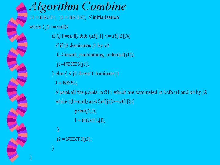
Algorithm Combine J 1 = BEG 31; j 2 = BEG 32; // initialization while ( j 2 != null){ if ((j 1!=null) && (u 3[j 1] <= u 3[j 2])){ // if j 2 dominates j 1 by u 3 L->insert_maintaining_order(u 4[j 1]); j 1=NEXT 3[j 1]; } else { // j 2 doesn’t dominate j 1 l = BEGL; // print all the points in S 11 which are dominated in both u 3 and u 4 by j 2 while ((l!=null) and (u 4[j 2]>=u 4[l])){ print(j 2, l); l = NEXTL[l]; } j 2 = NEXT 3[j 2]; } }

Example

The Crucial task of the procedure How can we insert u 4[j 1] into L maintaining sorted order efficiently? w The naive approach would yield time w Using AVL Trees we can achieve O(|S 1|log|S 11|) w We can take advantage of the fact that the points are known in advance to achieve O(|S 1|) total time w

Creating Schedule Of Insertion Into L in O(|S 11|) The Basic Idea : Let’s take a look at the point p in S 11 which has the highest u 3 value. We reach p after we processed all the other points from S 11. It should be placed in L after PRED 4[L] w Thus we can use PRED 4 from the QTL in order to determine the schedule of insertion into L w

Algorithm insertion schedule l = last(u 3 list) while ( PRED 3[l] != BEG 3 ) { NEXT 4[PRED 4[l]] = NEXT 4[l]; PRED 4[NEXT 4[l]] = PRED 4[l]; l = PRED 3[l]; } w Final L is PREV 4

Example

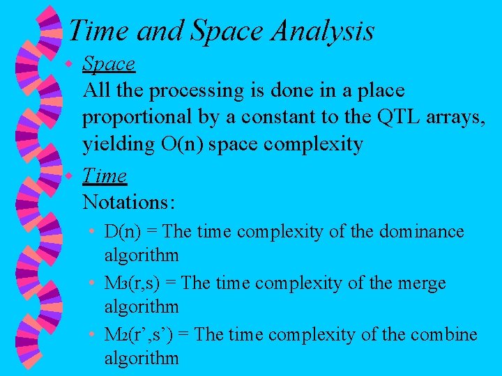
Time and Space Analysis Space All the processing is done in a place proportional by a constant to the QTL arrays, yielding O(n) space complexity w Time Notations: w • D(n) = The time complexity of the dominance algorithm • M 3(r, s) = The time complexity of the merge algorithm • M 2(r’, s’) = The time complexity of the combine algorithm

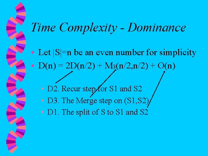
Time Complexity - Dominance Let |S|=n be an even number for simplicity w D(n) = 2 D(n/2) + M 3(n/2, n/2) + O(n) w • D 2. Recur step for S 1 and S 2 • D 3. The Merge step on (S 1, S 2) • D 1. The split of S to S 1 and S 2

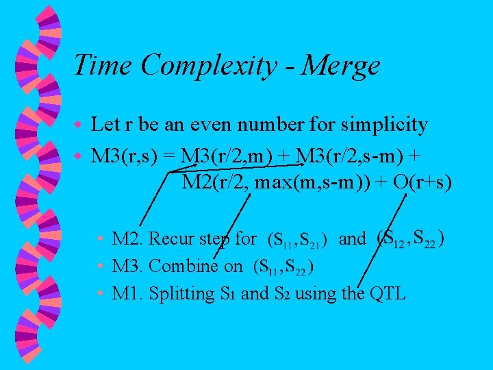
Time Complexity - Merge Let r be an even number for simplicity w M 3(r, s) = M 3(r/2, m) + M 3(r/2, s-m) + M 2(r/2, max(m, s-m)) + O(r+s) w • M 2. Recur step for and • M 3. Combine on • M 1. Splitting S 1 and S 2 using the QTL

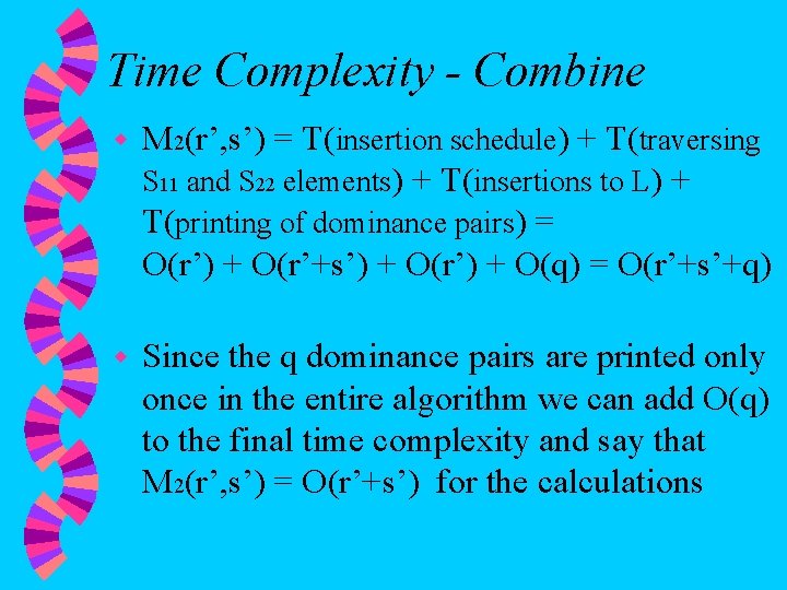
Time Complexity - Combine w M 2(r’, s’) = T(insertion schedule) + T(traversing S 11 and S 22 elements) + T(insertions to L) + T(printing of dominance pairs) = O(r’) + O(r’+s’) + O(r’) + O(q) = O(r’+s’+q) w Since the q dominance pairs are printed only once in the entire algorithm we can add O(q) to the final time complexity and say that M 2(r’, s’) = O(r’+s’) for the calculations

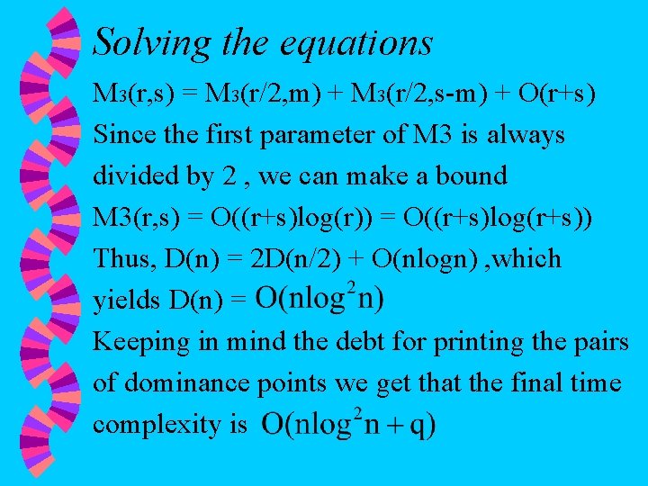
Solving the equations M 3(r, s) = M 3(r/2, m) + M 3(r/2, s-m) + O(r+s) Since the first parameter of M 3 is always divided by 2 , we can make a bound M 3(r, s) = O((r+s)log(r)) = O((r+s)log(r+s)) Thus, D(n) = 2 D(n/2) + O(nlogn) , which yields D(n) = Keeping in mind the debt for printing the pairs of dominance points we get that the final time complexity is

Next Steps There are variations of this algorithm which improve the time complexity on account of the space complexity