An Extension of Stochastic Greens Function Method to

An Extension of Stochastic Green’s Function Method to Long-Period Strong Ground-motion Simulation Y. Hisada and J. Bielak

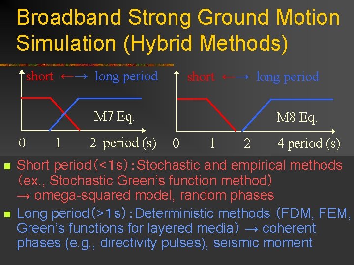
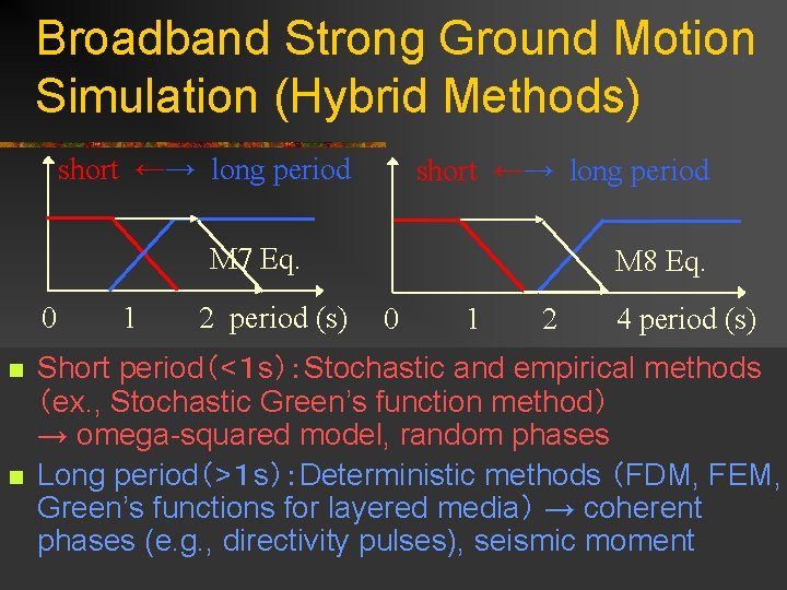
Broadband Strong Ground Motion Simulation (Hybrid Methods) short ←→ long period M 7 Eq. 0 　 1 n n 2 period (s) M 8 Eq. 0 　 1 2　 4 period (s) Short period（<１ s）：Stochastic and empirical methods （ex. , Stochastic Green’s function method）　　　　　　　 → omega-squared model, random phases Long period（>１ s）：Deterministic methods （FDM, FEM, Green’s functions for layered media） → coherent phases (e. g. , directivity pulses), seismic moment

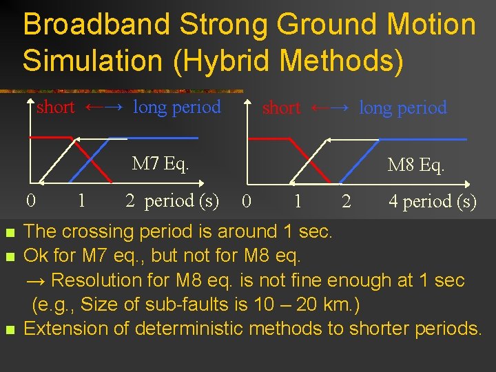
Broadband Strong Ground Motion Simulation (Hybrid Methods) short ←→ long period M 7 Eq. 0 　 1 n n n 2 period (s) M 8 Eq. 0 　 1 2　 4 period (s) The crossing period is around 1 sec. Ok for M 7 eq. , but not for M 8 eq. → Resolution for M 8 eq. is not fine enough at 1 sec (e. g. , Size of sub-faults is 10 – 20 km. ) Extension of deterministic methods to shorter periods.

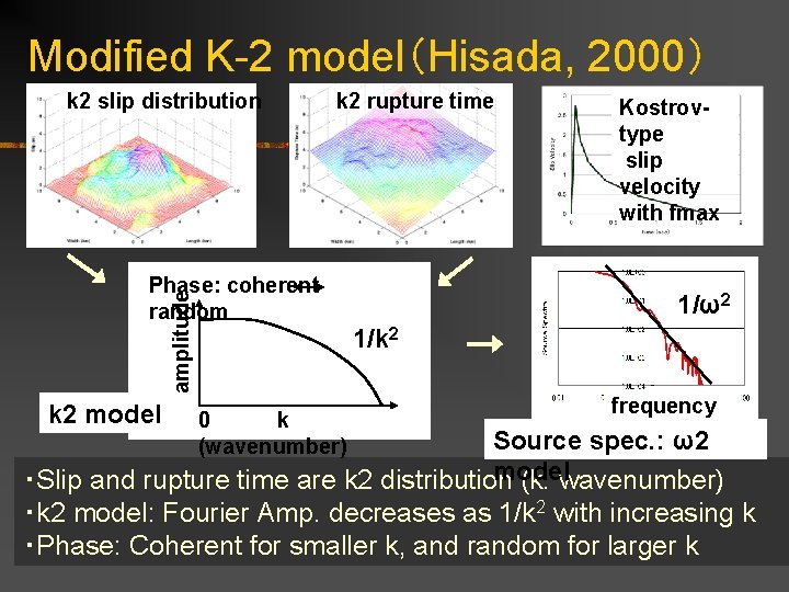
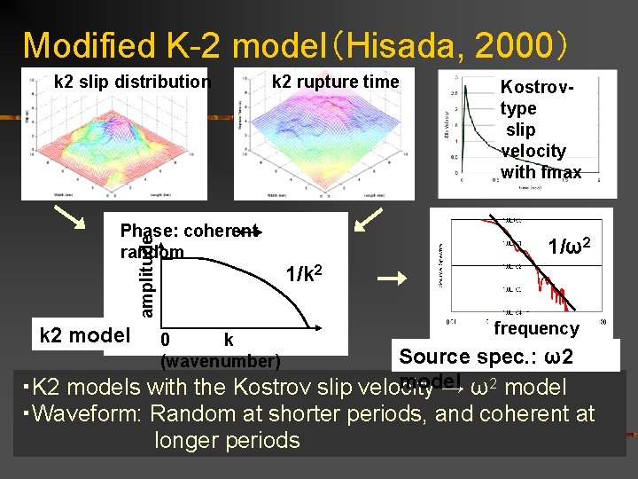
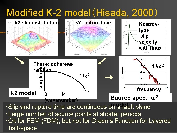
Modified K-2 model（Hisada, 2000） k 2 slip distribution k 2 rupture time amplitude Phase: coherent random k 2 model 0 k (wavenumber) Kostrovtype slip velocity with fmax 1/ω2 1/k 2 frequency Source spec. : ω2 model ・Slip and rupture time are k 2 distribution (k: wavenumber) ・k 2 model: Fourier Amp. decreases as 1/k 2 with increasing k ・Phase: Coherent for smaller k, and random for larger k

Modified K-2 model（Hisada, 2000） k 2 slip distribution k 2 rupture time amplitude Phase: coherent random k 2 model 0 k (wavenumber) Kostrovtype slip velocity with fmax 1/ω2 1/k 2 frequency Source spec. : ω2 model ・K 2 models with the Kostrov slip velocity → ω2 model ・Waveform: Random at shorter periods, and coherent at longer periods

Modified K-2 model（Hisada, 2000） k 2 slip distribution k 2 rupture time amplitude Phase: coherent random k 2 model 0 k (wavenumber) Kostrovtype slip velocity with fmax 1/ω2 1/k 2 frequency Source spec. : ω2 model ・Slip and rupture time are continuous on a fault plane ・Large number of source points at shorter periods ・Ok for FEM (FDM), but not for Green’s Function for Layered half-space

Broadband Strong Ground Motion Simulation (Hybrid Methods) short ←→ long period M 7 Eq. 0 　 1 n n 2 period (s) M 8 Eq. 0 　 1 2　 4 period (s) Short period（<１ s）：Stochastic and empirical methods （ex. , Stochastic Green’s function method）　　　　　　　 → omega-squared model, random phases Long period（>１ s）：Deterministic methods （FDM, FEM, Green’s functions for layered media） → coherent phases (e. g. , directivity pulses), seismic moment

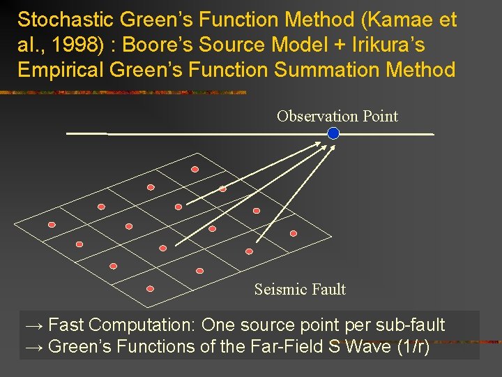
Stochastic Green’s Function Method (Kamae et al. , 1998) : Boore’s Source Model + Irikura’s Empirical Green’s Function Summation Method Observation Point Seismic Fault → Fast Computation: One source point per sub-fault → Green’s Functions of the Far-Field S Wave (1/r)

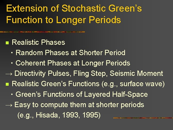
Extension of Stochastic Green’s Function to Longer Periods Realistic Phases 　・ Random Phases at Shorter Period 　・ Coherent Phases at Longer Periods → Directivity Pulses, Fling Step, Seismic Moment n Realistic Green’s Functions (e. g. , surface wave) 　・ Green’s Functions of Layered Half-Space → Easy to compute them at shorter periods (e. g. , Hisada, 1993, 1995) n

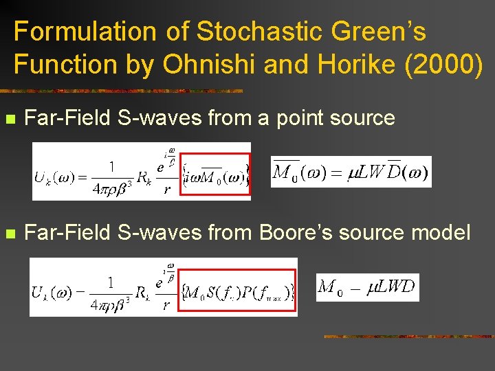
Formulation of Stochastic Green’s Function by Ohnishi and Horike (2000) n Far-Field S-waves from a point source n Far-Field S-waves from Boore’s source model

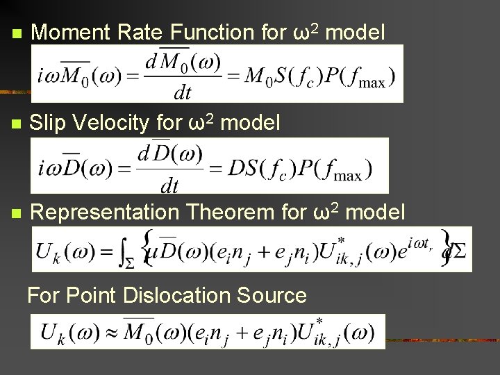
n Moment Rate Function for ω2 model n Slip Velocity for ω2 model n Representation Theorem for ω2 model For Point Dislocation Source

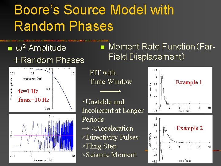
Boore’s Source Model with Random Phases n ω2 Amplitude ＋Random Phases n Moment Rate Function（Far. Field Displacement） FIT with Time Window fc=1 Hz fmax=10 Hz ・Unstable and Incoherent at Longer Periods → ○Acceleration ×Directivity Pulses ×Fling Step ×Seismic Moment Example 1 Example 2

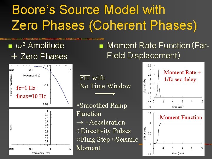
Boore’s Source Model with Zero Phases (Coherent Phases) ω2 Amplitude ＋ Zero Phases n fc=1 Hz fmax=10 Hz n Moment Rate Function（Far. Field Displacement） FIT with No Time Window ・Smoothed Ramp Function → ×Acceleration ○Directivity Pulses ○Fling Step ○Seismic Moment Rate + 1/fc sec delay Moment Function

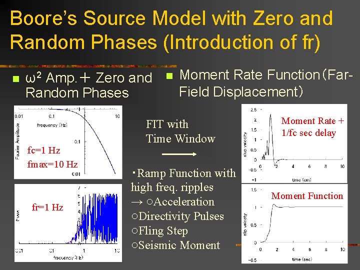
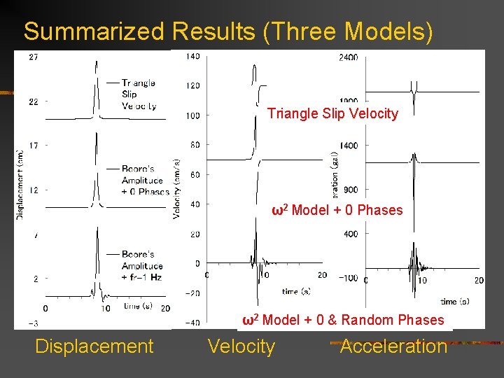
Boore’s Source Model with Zero and Random Phases (Introduction of fr) n ω2 Amp. ＋ Zero and Random Phases fc=1 Hz fmax=10 Hz fr=1 Hz n Moment Rate Function（Far. Field Displacement） FIT with Time Window ・Ramp Function with high freq. ripples → ○Acceleration ○Directivity Pulses ○Fling Step ○Seismic Moment Rate + 1/fc sec delay Moment Function

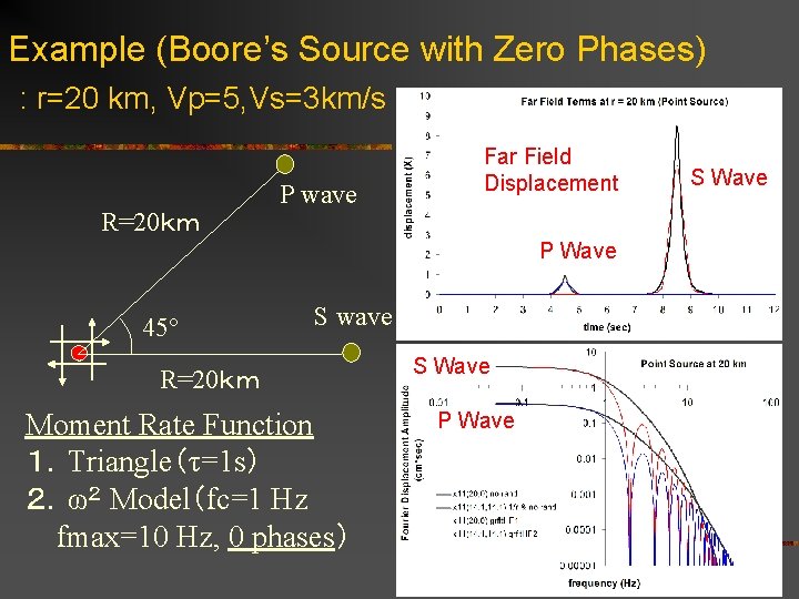
Example (Boore’s Source with Zero Phases) : r=20 km, Vp=5, Vs=3 km/s R=20ｋｍ P wave Far Field Displacement P Wave 45° S wave R=20ｋｍ Moment Rate Function １．Triangle（τ=1 s） ２．ω２ Model（fc=1 Hz fmax=10 Hz, 0 phases） S Wave P Wave S Wave

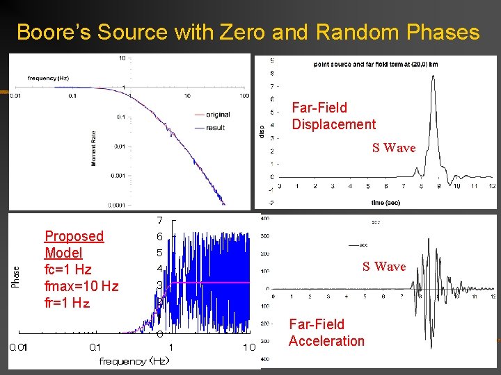
Boore’s Source with Zero and Random Phases Far-Field Displacement S Wave Proposed Model fc=1 Hz fmax=10 Hz fr=1 Hｚ S Wave Far-Field Acceleration

Summarized Results (Three Models) Triangle Slip Velocity ω2 Model + 0 Phases ω2 Model + 0 & Random Phases Displacement　　 Velocity　 　 Acceleration

Summary n n We extended a stochastic Green’s function method to longer periods in order to simulate coherent waves, by introducing zero phases at frequencies smaller than fr (a corner frequency). We can easily incorporate this method with more realistic Green’s functions, such as those of layered half-spaces.