An Evaluation of Multiresolution Storage for Sensor Networks
- Slides: 21

An Evaluation of Multi-resolution Storage for Sensor Networks Deepak Ganesan, Ben Greenstein, Denis Perelyubskiy, Deborah Estrin (UCLA) , John Heidemann (USC/ISI) Presenter: Vijay Sundaram 1

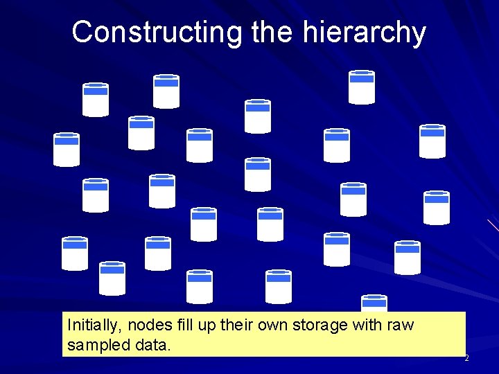
Constructing the hierarchy Initially, nodes fill up their own storage with raw sampled data. 2

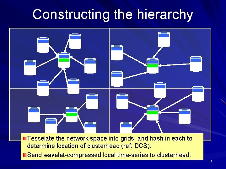
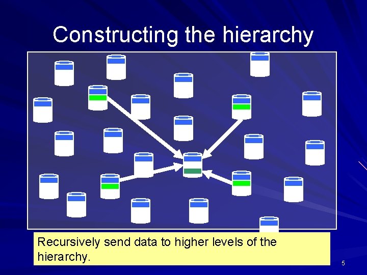
Constructing the hierarchy Tesselate the network space into grids, and hash in each to determine location of clusterhead (ref: DCS). Send wavelet-compressed local time-series to clusterhead. 3

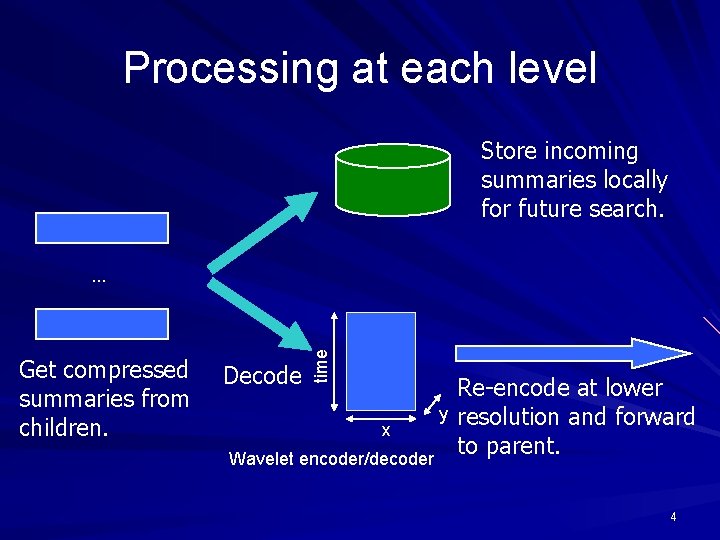
Processing at each level Store incoming summaries locally for future search. Get compressed summaries from children. Decode time … x Wavelet encoder/decoder y Re-encode at lower resolution and forward to parent. 4

Constructing the hierarchy Recursively send data to higher levels of the hierarchy. 5

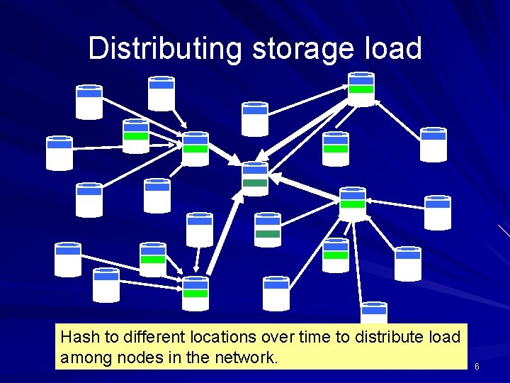
Distributing storage load Hash to different locations over time to distribute load among nodes in the network. 6

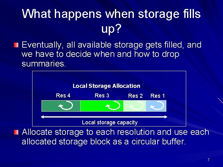
What happens when storage fills up? Eventually, all available storage gets filled, and we have to decide when and how to drop summaries. Local Storage Allocation Res 4 Res 3 Res 2 Res 1 Local storage capacity Allocate storage to each resolution and use each allocated storage block as a circular buffer. 7

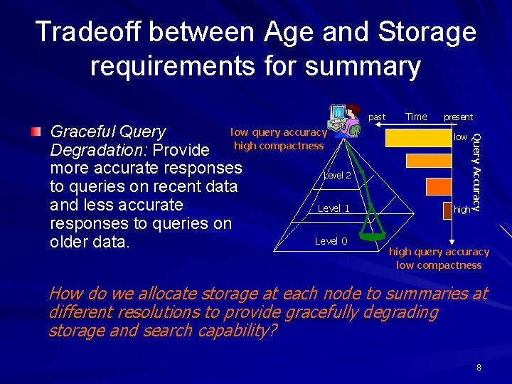
Tradeoff between Age and Storage requirements for summary Time present low high Query Accuracy low query accuracy Graceful Query Degradation: Provide high compactness more accurate responses Level 2 to queries on recent data and less accurate Level 1 responses to queries on Level 0 older data. past high query accuracy low compactness How do we allocate storage at each node to summaries at different resolutions to provide gracefully degrading storage and search capability? 8

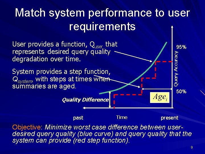
Match system performance to user requirements System provides a step function, Qsystem, with steps at times when summaries are aged. 95% Query Accuracy User provides a function, Quser that represents desired query quality degradation over time. 50% Quality Difference past Time present Objective: Minimize worst case difference between userdesired query quality (blue curve) and query quality that the system can provide (red step function). 9

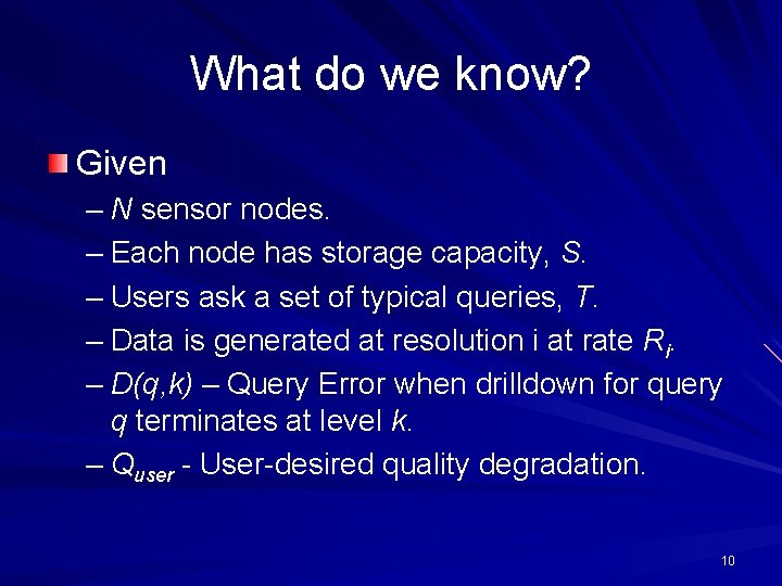
What do we know? Given – N sensor nodes. – Each node has storage capacity, S. – Users ask a set of typical queries, T. – Data is generated at resolution i at rate Ri. – D(q, k) – Query Error when drilldown for query q terminates at level k. – Quser - User-desired quality degradation. 10

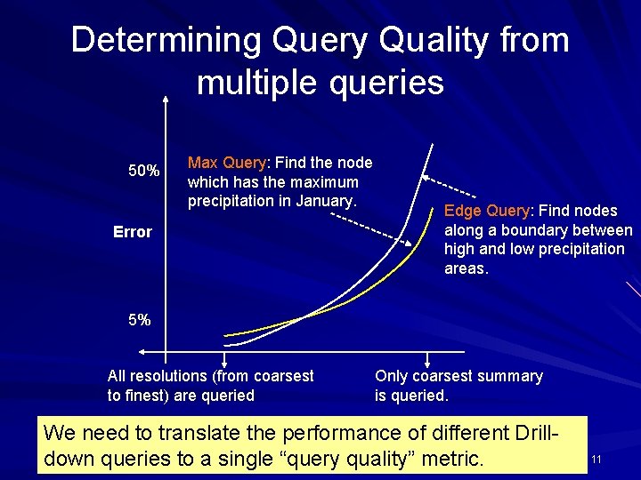
Determining Query Quality from multiple queries 50% Max Query: Find the node which has the maximum precipitation in January. Error Edge Query: Find nodes along a boundary between high and low precipitation areas. 5% All resolutions (from coarsest to finest) are queried Only coarsest summary is queried. We need to translate the performance of different Drilldown queries to a single “query quality” metric. 11

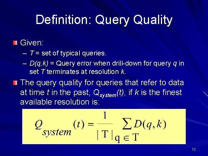
Definition: Query Quality Given: – T = set of typical queries. – D(q, k) = Query error when drill-down for query q in set T terminates at resolution k. The query quality for queries that refer to data at time t in the past, Qsystem(t), if k is the finest available resolution is: 12

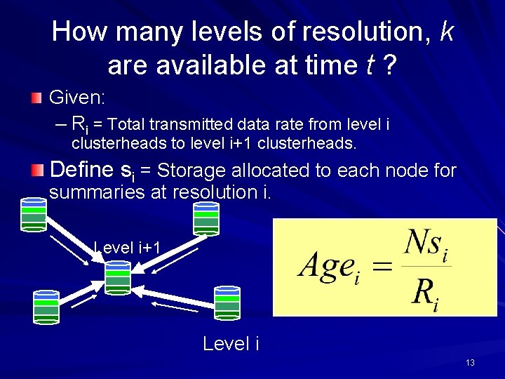
How many levels of resolution, k are available at time t ? Given: – Ri = Total transmitted data rate from level i clusterheads to level i+1 clusterheads. Define si = Storage allocated to each node for summaries at resolution i. Level i+1 Level i 13

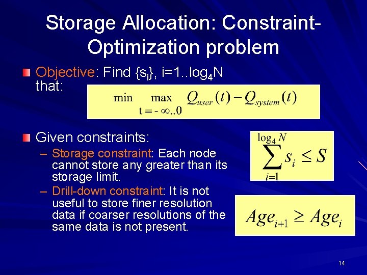
Storage Allocation: Constraint. Optimization problem Objective: Find {si}, i=1. . log 4 N that: Given constraints: – Storage constraint: Each node cannot store any greater than its storage limit. – Drill-down constraint: It is not useful to store finer resolution data if coarser resolutions of the same data is not present. 14

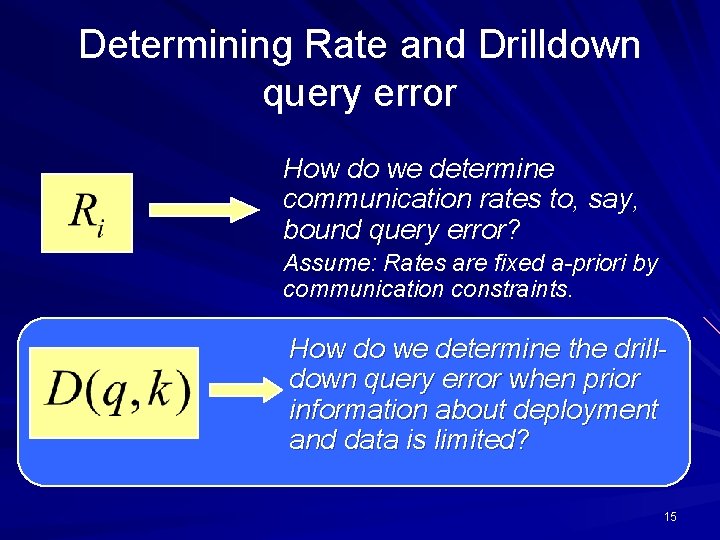
Determining Rate and Drilldown query error How do we determine communication rates to, say, bound query error? Assume: Rates are fixed a-priori by communication constraints. How do we determine the drilldown query error when prior information about deployment and data is limited? 15

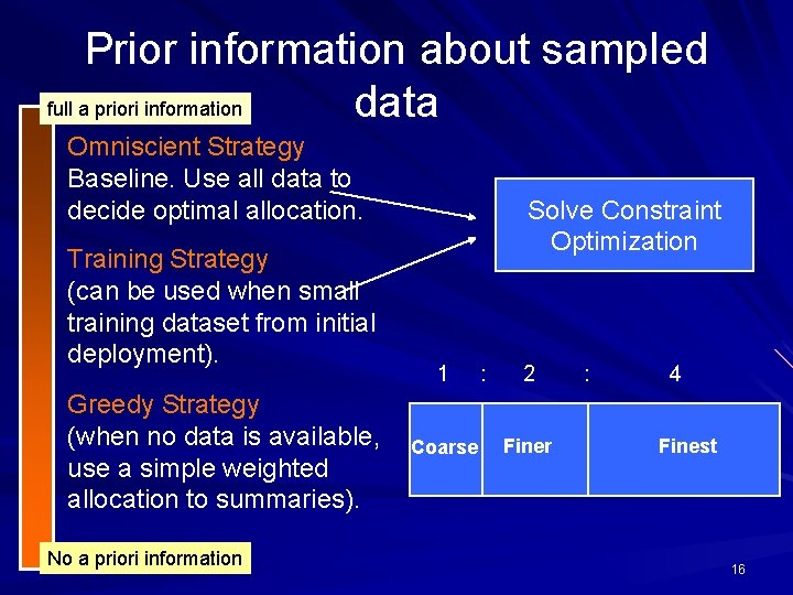
Prior information about sampled full a priori information data Omniscient Strategy Baseline. Use all data to decide optimal allocation. Training Strategy (can be used when small training dataset from initial deployment). Greedy Strategy (when no data is available, use a simple weighted allocation to summaries). No a priori information Solve Constraint Optimization 1 Coarse : 2 Finer : 4 Finest 16

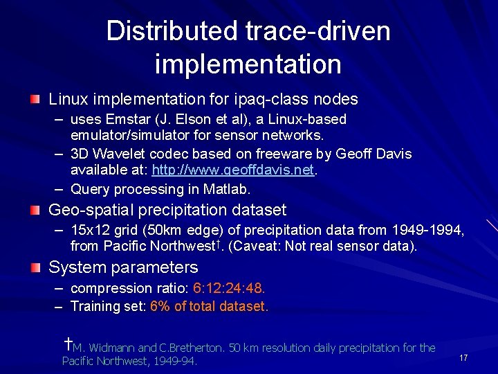
Distributed trace-driven implementation Linux implementation for ipaq-class nodes – uses Emstar (J. Elson et al), a Linux-based emulator/simulator for sensor networks. – 3 D Wavelet codec based on freeware by Geoff Davis available at: http: //www. geoffdavis. net. – Query processing in Matlab. Geo-spatial precipitation dataset – 15 x 12 grid (50 km edge) of precipitation data from 1949 -1994, from Pacific Northwest†. (Caveat: Not real sensor data). System parameters – compression ratio: 6: 12: 24: 48. – Training set: 6% of total dataset. †M. Widmann and C. Bretherton. 50 km resolution daily precipitation for the Pacific Northwest, 1949 -94. 17

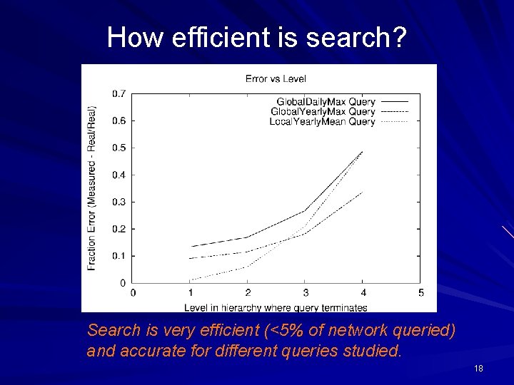
How efficient is search? Search is very efficient (<5% of network queried) and accurate for different queries studied. 18

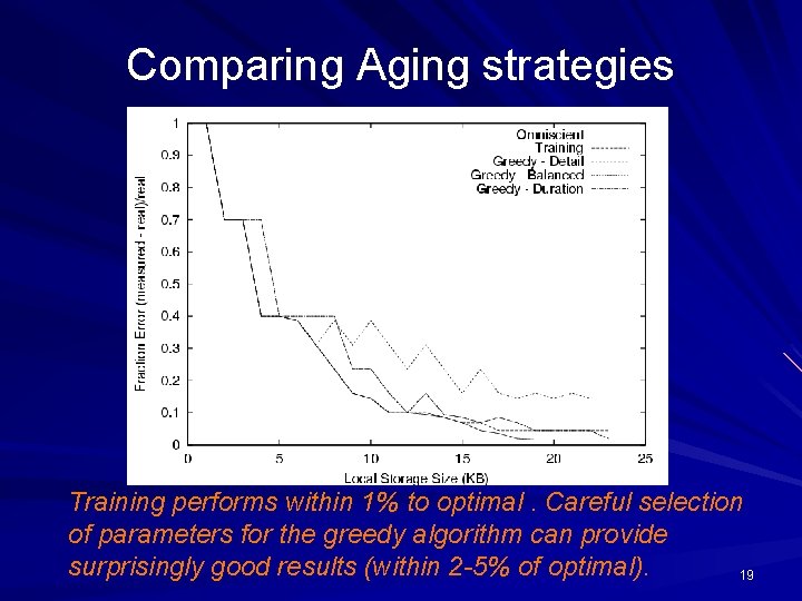
Comparing Aging strategies Training performs within 1% to optimal. Careful selection of parameters for the greedy algorithm can provide surprisingly good results (within 2 -5% of optimal). 19

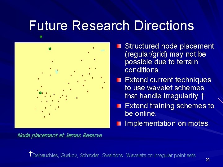
Future Research Directions Structured node placement (regular/grid) may not be possible due to terrain conditions. Extend current techniques to use wavelet schemes that handle irregularity †. Extend training schemes to be online. Implementation on motes. Node placement at James Reserve †Debauchies, Guskov, Schroder, Sweldons: Wavelets on irregular point sets 20

Summary Progressive aging of summaries can be used to support long-term spatio-temporal queries in resourceconstrained sensor network deployments. We describe two algorithms: a training-based algorithm that relies on the availability of training datasets, and a greedy algorithm can be used in the absence of such data. Our results show that – training performs close to optimal for the dataset that we study. – the greedy algorithm performs well for a well-chosen summary weighting parameter. 21