An Engineers Guide to MATLAB Chapter 5 AN

An Engineer’s Guide to MATLAB Chapter 5 – Objectives • Describe how functions are created and give numerous examples of MATLAB functions that are frequently used to obtain numerical solutions to engineering problems. Copyright © Edward B. Magrab 2009 2

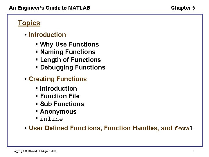
An Engineer’s Guide to MATLAB Chapter 5 Topics • Introduction § Why Use Functions § Naming Functions § Length of Functions § Debugging Functions • Creating Functions § Introduction § Function File § Sub Functions § Anonymous § inline • User Defined Functions, Function Handles, and feval Copyright © Edward B. Magrab 2009 3

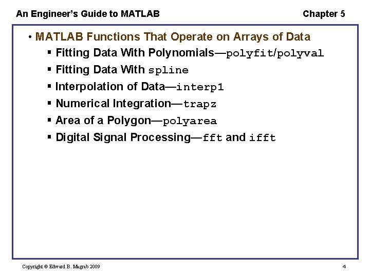
An Engineer’s Guide to MATLAB Chapter 5 • MATLAB Functions That Operate on Arrays of Data § Fitting Data With Polynomials—polyfit/polyval § Fitting Data With spline § Interpolation of Data—interp 1 § Numerical Integration—trapz § Area of a Polygon—polyarea § Digital Signal Processing—fft and ifft Copyright © Edward B. Magrab 2009 4

An Engineer’s Guide to MATLAB Chapter 5 • MATLAB Functions That Require User-Created Functions § Zeros of Functions—fzero and roots/poly § Numerical Integration—quadl and dblquad § Numerical Solutions of Ordinary Differential Equations —ode 45 § Numerical Solutions of Ordinary Differential Equations —bvp 4 c § Numerical Solutions of Delay Differential Equations—dde 23 § Numerical Solutions of One-dimensional Parabolicelliptic Partial Differential Equations—pdepe § Local Minimum of a Function—fminbnd § Numerical Solutions of Nonlinear Equations—fsolve • Symbolic Toolbox and the Creation of Functions Copyright © Edward B. Magrab 2009 5

An Engineer’s Guide to MATLAB Chapter 5 Introduction – Function files are script files that create their own local and independent workspace within MATLAB. Variables defined within a function are local to that function. They neither affect nor are they affected by the same variable names being used in any script or other function. All of MATLAB’s functions are of this type. The exception is those variables that are designated global variables. The first non-comment line of a function must follow a prescribed format. Copyright © Edward B. Magrab 2009 6

An Engineer’s Guide to MATLAB Chapter 5 Why Use Functions – • Avoid duplicate code. • Limit the effect of changes to specific sections of a program. • Promote program reuse. • Reduce the complexity of the overall program by making it more readable and manageable. • Isolate complex operations. • Improve portability. • Make debugging and error isolation easier. • Improve performance because each function can be “optimized”. Copyright © Edward B. Magrab 2009 7

An Engineer’s Guide to MATLAB Chapter 5 Naming Functions • The names of functions should be chosen so that they are meaningful and indicate what the function does. • Typical lengths of function names are between 9 and 20 characters and should employ standard or consistent conventions. • The proper choice of function names can also minimize the use of comments within the function itself. Copyright © Edward B. Magrab 2009 8

An Engineer’s Guide to MATLAB Chapter 5 Length of Functions • The length of a function can vary from two lines of code to hundreds of lines of code. • The length of a function should be governed, in part, by its functional cohesion – § The degree to which it does one thing and not anything else. • A function can be created with numerous highly cohesive functions to create another cohesive function. • Highly cohesive functions are reliable – § lower error rate • When functions have a low degree of cohesion, one often encounters difficulty in isolating errors. Copyright © Edward B. Magrab 2009 9

An Engineer’s Guide to MATLAB Chapter 5 • The compartmentalization brought about by the use of functions also tends to minimize the unintended use of data by portions of the program, because data to each function is provided only on a need-to-know basis. Copyright © Edward B. Magrab 2009 10

An Engineer’s Guide to MATLAB Chapter 5 Four Ways to Create Functions Function file Created by the function command, saved in a file, and subsequently accessed by scripts and functions or from the command window. Sub function When the function keyword is used more than once in a function file, then all the additional functions created after the first function keyword are called sub functions. The sub functions are only accessible by the main function of the function file and the other sub functions within the main function file. Copyright © Edward B. Magrab 2009 11

An Engineer’s Guide to MATLAB Chapter 5 Sub function - continued They are used to reduce function file proliferation while maintaining the features and uses of a function. Anonymous function A means of creating functions for simple expressions without having to create M-files or sub functions. It is accessible only from the script or function in which it was created. An anonymous function can appear in another anonymous function. An anonymous function doesn't have to be saved in a separate file. Copyright © Edward B. Magrab 2009 12

An Engineer’s Guide to MATLAB Chapter 5 inline function Created with the inline command limited to one MATLAB expression. It is accessible only from the script or function in which it was created. The MATLAB expression can not refer to other inline functions or sub functions. Copyright © Edward B. Magrab 2009 13

An Engineer’s Guide to MATLAB Chapter 5 Function File – • A function that is going to reside in a function file has at least two lines of program code. § The first line has a format required by MATLAB. • There is no terminating character or expression for the function program such as the end statement. • The name of the M-file should be the same as the name of the function, except that the file name has the extension “. m”. Copyright © Edward B. Magrab 2009 14

An Engineer’s Guide to MATLAB Chapter 5 The number of variables and their type (scalar, vector, matrix, string, cell) that are brought in and out of the function are controlled by the function interface, which is the first non-comment line of the function program. In general, a function file will consist of the interface line, some comments and one or more expressions as shown below. The interface has the general form: Copyright © Edward B. Magrab 2009 15

An Engineer’s Guide to MATLAB Chapter 5 function [Output. Variables] = Function. Name(Input. Variables) % Comments Expression(s) where Output. Variables is a comma-separated list of the names of the output variables. Input. Variables is a comma-separated list of the names of the input variables. The function file may be stored in any directory and has the file name Function. Name. m function [a, b, …] = Function. Name(V 1, V 2, V 3, …) Copyright © Edward B. Magrab 2009 16

An Engineer’s Guide to MATLAB Chapter 5 Special Case 1 Functions can be used to create a figure, to display annotated data to the command window, or to write data to files. In these cases, no values are transferred back to the calling program, which is a script or another function that uses this function in one or more of its expressions. In this case, the function interface line becomes function Function. Name(Input. Variables) function [a, b, …] = Function. Name(V 1, V 2, V 3, …) Copyright © Edward B. Magrab 2009 17

An Engineer’s Guide to MATLAB Chapter 5 Special Case 2 When a function is used only to store data in a prescribed manner, the function does not require any input arguments. In this case, the function interface line has the form function [Output. Variables] = Function. Name function [a, b, …] = Function. Name(V 1, V 2, V 3, …) Copyright © Edward B. Magrab 2009 18

An Engineer’s Guide to MATLAB Chapter 5 Special Case 3 When a function converts a script to a main function so that one can decrease the number of function M-files, the function interface line has the form function Function. Name function [a, b, …] = Function. Name(V 1, V 2, V 3, …) Copyright © Edward B. Magrab 2009 19

An Engineer’s Guide to MATLAB Chapter 5 About Functions – There are several concepts that must be understood to correctly create functions. • The variable names used in the function definition do not have to match the corresponding names when the function is called from the command window, a script, or another function. • It is the locations of the input variables within the argument list inside the parentheses that govern the transfer of information—that is, the first argument in the calling statement transfers its value(s) to the first argument in the function interface line, and so on. function Function. Name(V 1, V 2, V 3, …) Copyright © Edward B. Magrab 2009 20

An Engineer’s Guide to MATLAB Chapter 5 • The names selected for each argument are local to the function program and have meaning only within the context of the function program. • The same names can be used in an entirely different context in the script file that calls this function or in another function used by this function. § However, the names appearing for each input variable of the function statement must be the same type, either scalar, vector, matrix, cell, or string, in the calling program as in the function program in order for the function’s expressions to work as intended. • The variable names are not local to the function only when they have been assigned as global variables using global Copyright © Edward B. Magrab 2009 function Function. Name(V 1, V 2, V 3, …) 21

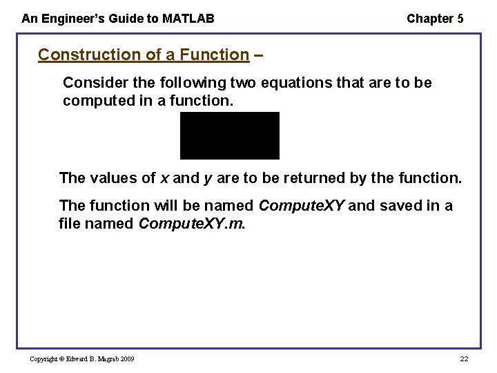
An Engineer’s Guide to MATLAB Chapter 5 Construction of a Function – Consider the following two equations that are to be computed in a function. The values of x and y are to be returned by the function. The function will be named Compute. XY and saved in a file named Compute. XY. m. Copyright © Edward B. Magrab 2009 22

An Engineer’s Guide to MATLAB Chapter 5 function [x, y] = Compute. XY(t, a, b, c) % Computation of % x = cos(at)+b % y = |x|+c % Scalars: a, b, c % Vectors: t, x, y x = cos(a*t)+b; y = abs(x)+c; When one types in the MATLAB command window help Compute. XY Computation of the following is displayed x = cos(at)+b y = |x|+c Scalars: a, b, c Vectors: t, x, y Copyright © Edward B. Magrab 2009 23

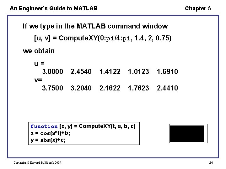
An Engineer’s Guide to MATLAB Chapter 5 If we type in the MATLAB command window [u, v] = Compute. XY(0: pi/4: pi, 1. 4, 2, 0. 75) we obtain u= 3. 0000 v= 3. 7500 2. 4540 1. 4122 1. 0123 1. 6910 3. 2040 2. 1622 1. 7623 2. 4410 function [x, y] = Compute. XY(t, a, b, c) x = cos(a*t)+b; y = abs(x)+c; Copyright © Edward B. Magrab 2009 24

An Engineer’s Guide to MATLAB Chapter 5 Variations of the function statement [u, v]

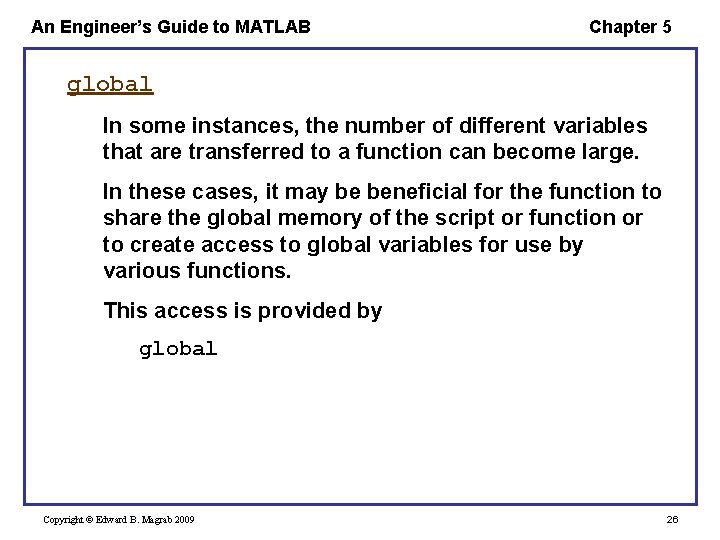
An Engineer’s Guide to MATLAB Chapter 5 global In some instances, the number of different variables that are transferred to a function can become large. In these cases, it may be beneficial for the function to share the global memory of the script or function or to create access to global variables for use by various functions. This access is provided by global Copyright © Edward B. Magrab 2009 26

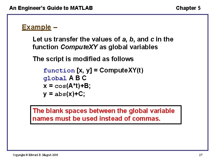
An Engineer’s Guide to MATLAB Chapter 5 Example – Let us transfer the values of a, b, and c in the function Compute. XY as global variables The script is modified as follows function [x, y] = Compute. XY(t) global A B C x = cos(A*t)+B; y = abs(x)+C; The blank spaces between the global variable names must be used instead of commas. Copyright © Edward B. Magrab 2009 27

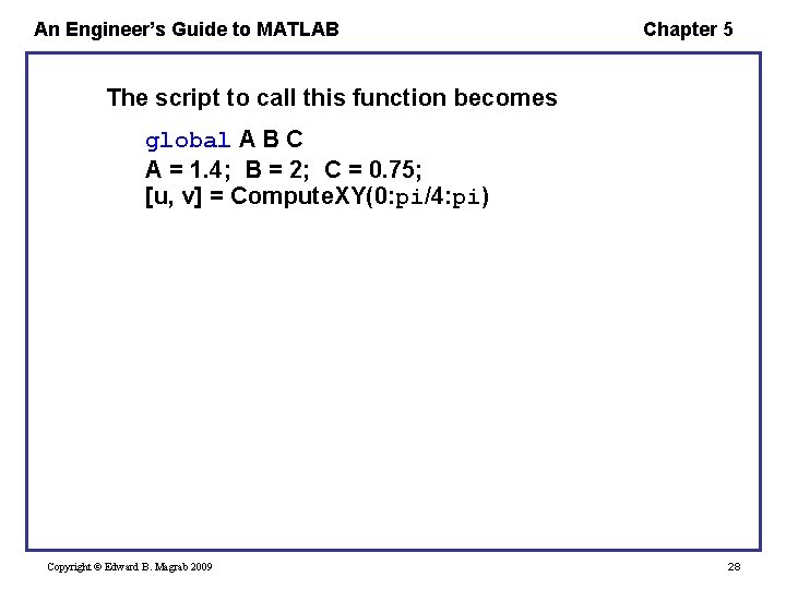
An Engineer’s Guide to MATLAB Chapter 5 The script to call this function becomes

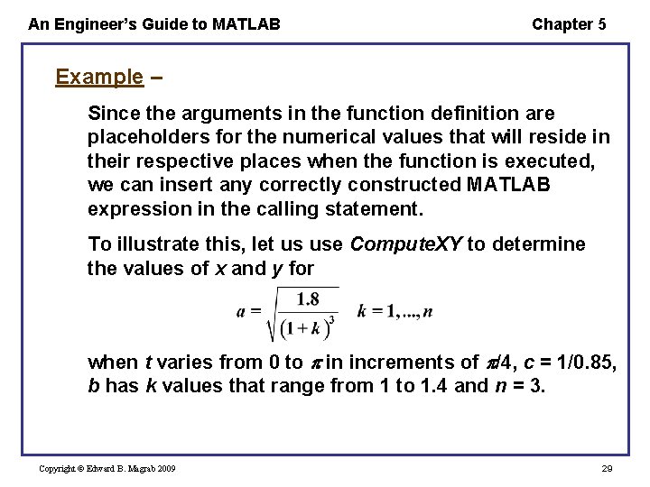
An Engineer’s Guide to MATLAB Chapter 5 Example – Since the arguments in the function definition are placeholders for the numerical values that will reside in their respective places when the function is executed, we can insert any correctly constructed MATLAB expression in the calling statement. To illustrate this, let us use Compute. XY to determine the values of x and y for when t varies from 0 to in increments of /4, c = 1/0. 85, b has k values that range from 1 to 1. 4 and n = 3. Copyright © Edward B. Magrab 2009 29

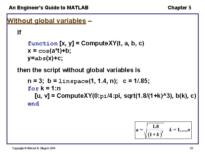
An Engineer’s Guide to MATLAB Chapter 5 Without global variables – If function [x, y] = Compute. XY(t, a, b, c) x = cos(a*t)+b; y=abs(x)+c; then the script without global variables is n = 3; b = linspace(1, 1. 4, n); c = 1/. 85; for k = 1: n [u, v] = Compute. XY(0: pi/4: pi, sqrt(1. 8/(1+k)^3), b(k), c) end Copyright © Edward B. Magrab 2009 30

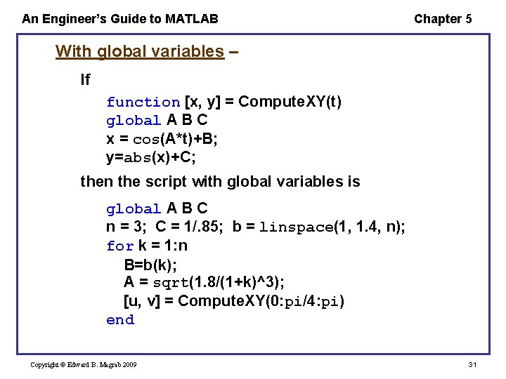
An Engineer’s Guide to MATLAB Chapter 5 With global variables – If function [x, y] = Compute. XY(t) global A B C x = cos(A*t)+B; y=abs(x)+C; then the script with global variables is global A B C n = 3; C = 1/. 85; b = linspace(1, 1. 4, n); for k = 1: n B=b(k); A = sqrt(1. 8/(1+k)^3); [u, v] = Compute. XY(0: pi/4: pi) end Copyright © Edward B. Magrab 2009 31

An Engineer’s Guide to MATLAB Chapter 5 Sub Functions • When the function keyword is used more than once in a function file, all the additional functions created after the first function key word are called sub functions. • The expressions comprising the first use of the function keyword is called the main function. § It is the only function that is accessible from the command window, scripts, and other function files. • The sub functions are accessible only to the main function and to other sub functions within the main function file. Copyright © Edward B. Magrab 2009 32

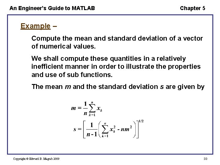
An Engineer’s Guide to MATLAB Chapter 5 Example – Compute the mean and standard deviation of a vector of numerical values. We shall compute these quantities in a relatively inefficient manner in order to illustrate the properties and use of sub functions. The mean m and the standard deviation s are given by Copyright © Edward B. Magrab 2009 33

An Engineer’s Guide to MATLAB Chapter 5 function [m, s] = Mean. Std. Dev(dat) n = length(dat); m = meen(dat, n); s = stdev(dat, n); function m = meen(v, n) m = sum(v)/n; % Main function % Sub function sd = stdev(v, n) % Sub function m = meen(v, n); % Calls a sub function sd = sqrt((sum(v. ^2)-n*m^2)/(n-1)); A script that uses this function and sub functions is v = [1, 2 , 3, 4]; [m, s] = Mean. Std. Dev(v) Copyright © Edward B. Magrab 2009 34

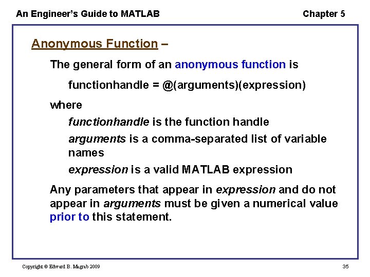
An Engineer’s Guide to MATLAB Chapter 5 Anonymous Function – The general form of an anonymous function is functionhandle = @(arguments)(expression) where functionhandle is the function handle arguments is a comma-separated list of variable names expression is a valid MATLAB expression Any parameters that appear in expression and do not appear in arguments must be given a numerical value prior to this statement. Copyright © Edward B. Magrab 2009 35

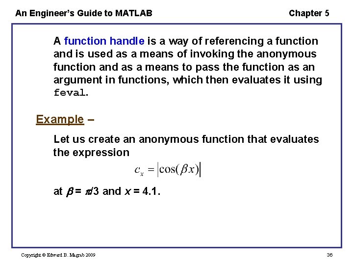
An Engineer’s Guide to MATLAB Chapter 5 A function handle is a way of referencing a function and is used as a means of invoking the anonymous function and as a means to pass the function as an argument in functions, which then evaluates it using feval. Example – Let us create an anonymous function that evaluates the expression at = /3 and x = 4. 1. Copyright © Edward B. Magrab 2009 36

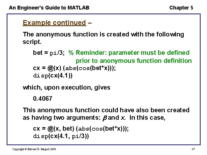
An Engineer’s Guide to MATLAB Chapter 5 Example continued – The anonymous function is created with the following script. bet = pi/3; % Reminder: parameter must be defined prior to anonymous function definition cx = @(x) (abs(cos(bet*x))); disp(cx(4. 1)) which, upon execution, gives 0. 4067 This anonymous function could have also been created as having two arguments: and x. In this case, cx = @(x, bet) (abs(cos(bet*x))); disp(cx(4. 1, pi/3)) Copyright © Edward B. Magrab 2009 37

An Engineer’s Guide to MATLAB Chapter 5 Example continued – We can also use this anonymous function directly in another anonymous function. Let us create an anonymous function that determines the cube root. Then cx = @(x, bet) (abs(cos(bet*x))); crt = @(x) (x^(1/3)); disp(crt(cx(4. 1, pi/3))) which, upon execution, results in 0. 7409 Copyright © Edward B. Magrab 2009 38

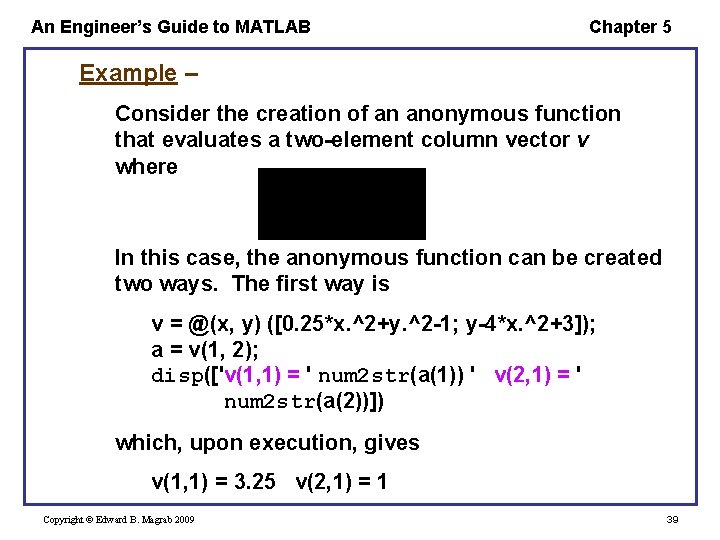
An Engineer’s Guide to MATLAB Chapter 5 Example – Consider the creation of an anonymous function that evaluates a two-element column vector v where In this case, the anonymous function can be created two ways. The first way is v = @(x, y) ([0. 25*x. ^2+y. ^2 -1; y-4*x. ^2+3]); a = v(1, 2); disp(['v(1, 1) = ' num 2 str(a(1)) ' v(2, 1) = ' num 2 str(a(2))]) which, upon execution, gives v(1, 1) = 3. 25 v(2, 1) = 1 Copyright © Edward B. Magrab 2009 39

An Engineer’s Guide to MATLAB Chapter 5 Example continued – The second way is v = @(xy) ([0. 25*xy(1). ^2+xy(2). ^2 -1; xy(2)-4*xy(1). ^2+3]); a = v([1, 2]); disp(['v(1, 1) = ' num 2 str(a(1)) ' v(2, 1) = ' num 2 str(a(2))]) where xy(1) = x = 1 and xy(2) = y = 2. Execution of this program produces the previous results. Copyright © Edward B. Magrab 2009 40

An Engineer’s Guide to MATLAB Chapter 5 inline • Can be created either in the command window, a script, or a function. • Is not saved in a separate file. • Limitations § Cannot call another inline function, but it can use a user-created function existing as a function file. § Is composed of only one expression. § It can bring back only one variable—that is, the form [u, v] is not allowed. § Any function requiring logic or multiple operations to arrive at the result cannot employ inline. Copyright © Edward B. Magrab 2009 41

An Engineer’s Guide to MATLAB Chapter 5 The general form of inline is Function. Name = inline('expression', 'p 1', 'p 2', …) where expression is any valid MATLAB expression converted to a string and p 1, p 2, … are the names of all the variables appearing in expression. All single quotes are required as shown. Copyright © Edward B. Magrab 2009 42

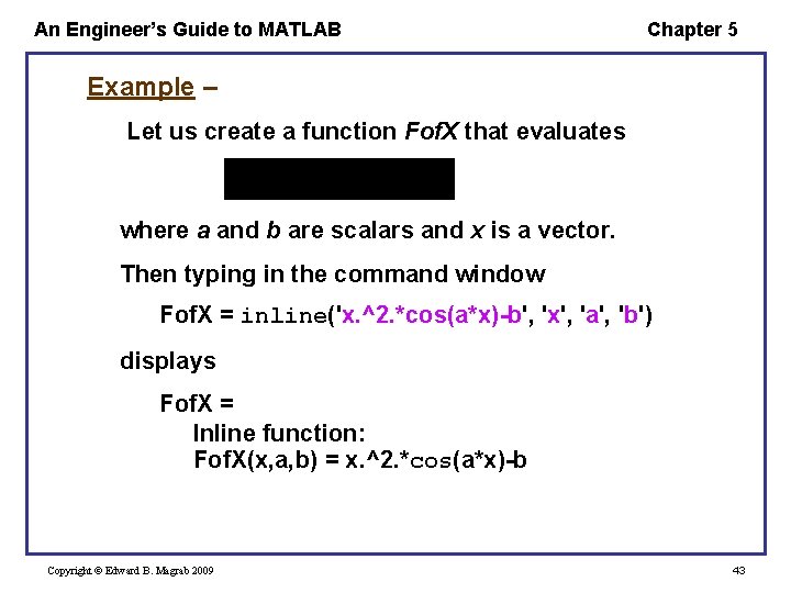
An Engineer’s Guide to MATLAB Chapter 5 Example – Let us create a function Fof. X that evaluates where a and b are scalars and x is a vector. Then typing in the command window Fof. X = inline('x. ^2. *cos(a*x)-b', 'x', 'a', 'b') displays Fof. X = Inline function: Fof. X(x, a, b) = x. ^2. *cos(a*x)-b Copyright © Edward B. Magrab 2009 43

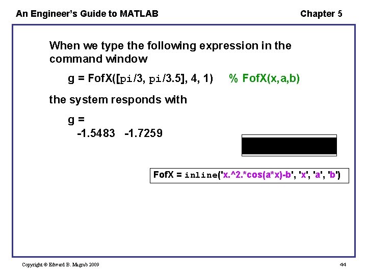
An Engineer’s Guide to MATLAB Chapter 5 When we type the following expression in the command window g = Fof. X([pi/3, pi/3. 5], 4, 1) % Fof. X(x, a, b) the system responds with g= -1. 5483 -1. 7259 Fof. X = inline('x. ^2. *cos(a*x)-b', 'x', 'a', 'b') Copyright © Edward B. Magrab 2009 44

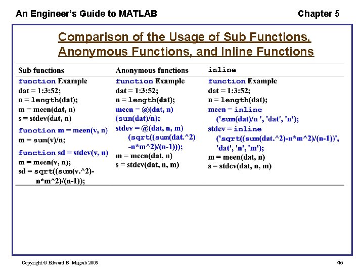
An Engineer’s Guide to MATLAB Chapter 5 Comparison of the Usage of Sub Functions,

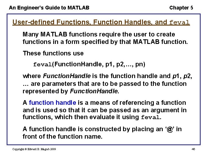
An Engineer’s Guide to MATLAB Chapter 5 User-defined Functions, Function Handles, and feval Many MATLAB functions require the user to create functions in a form specified by that MATLAB function. These functions use feval(Function. Handle, p 1, p 2, …, pn) where Function. Handle is the function handle and p 1, p 2, … are parameters that are to be passed to the function represented by Function. Handle. A function handle is a means of referencing a function and is used so that it can be passed as an argument in functions, which then evaluate it using feval. A function handle is constructed by placing an ‘@’ in front of the function name. Copyright © Edward B. Magrab 2009 46

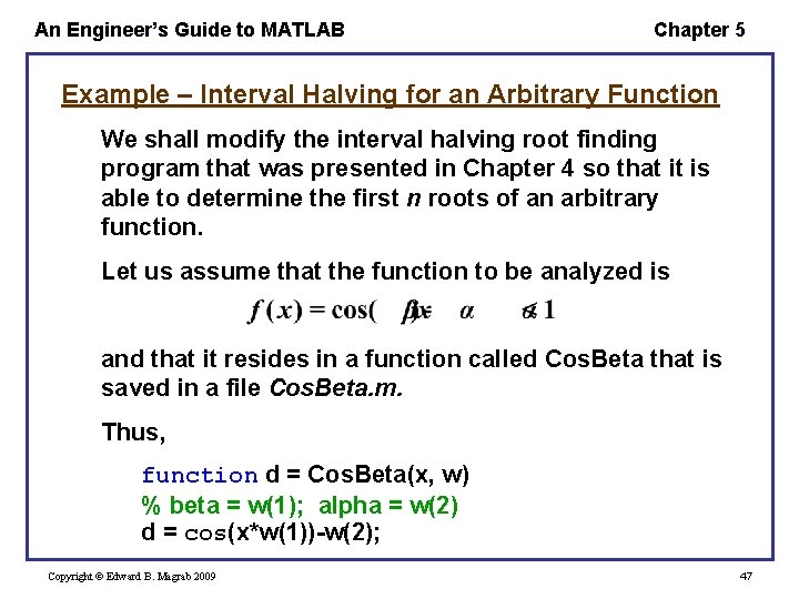
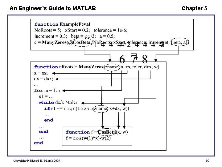
An Engineer’s Guide to MATLAB Chapter 5 Example – Interval Halving for an Arbitrary Function We shall modify the interval halving root finding program that was presented in Chapter 4 so that it is able to determine the first n roots of an arbitrary function. Let us assume that the function to be analyzed is and that it resides in a function called Cos. Beta that is saved in a file Cos. Beta. m. Thus, function d = Cos. Beta(x, w) % beta = w(1); alpha = w(2) d = cos(x*w(1))-w(2); Copyright © Edward B. Magrab 2009 47

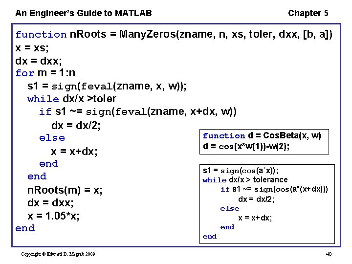
An Engineer’s Guide to MATLAB Chapter 5 function n. Roots = Many. Zeros(zname, n, xs, toler, dxx, [b, a]) x = xs; dx = dxx; for m = 1: n s 1 = sign(feval(zname, x, w)); while dx/x >toler if s 1 ~= sign(feval(zname, x+dx, w)) dx = dx/2; function d = Cos. Beta(x, w) else d = cos(x*w(1))-w(2); x = x+dx; end s 1 = sign(cos(a*x)); end while dx/x > tolerance if s 1 ~= sign(cos(a*(x+dx))) n. Roots(m) = x; dx = dx/2; dx = dxx; else x = 1. 05*x; x = x+dx; end end Copyright © Edward B. Magrab 2009 48

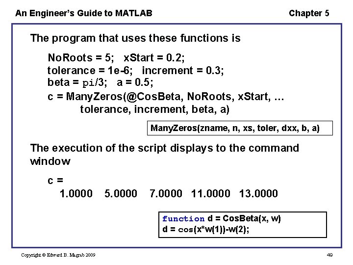
An Engineer’s Guide to MATLAB Chapter 5 The program that uses these functions is No. Roots = 5; x. Start = 0. 2; tolerance = 1 e-6; increment = 0. 3; beta = pi/3; a = 0. 5; c = Many. Zeros(@Cos. Beta, No. Roots, x. Start, … tolerance, increment, beta, a) Many. Zeros(zname, n, xs, toler, dxx, b, a) The execution of the script displays to the command window c= 1. 0000 5. 0000 7. 0000 11. 0000 13. 0000 function d = Cos. Beta(x, w) d = cos(x*w(1))-w(2); Copyright © Edward B. Magrab 2009 49

An Engineer’s Guide to MATLAB Copyright © Edward B. Magrab 2009 Chapter 5 50

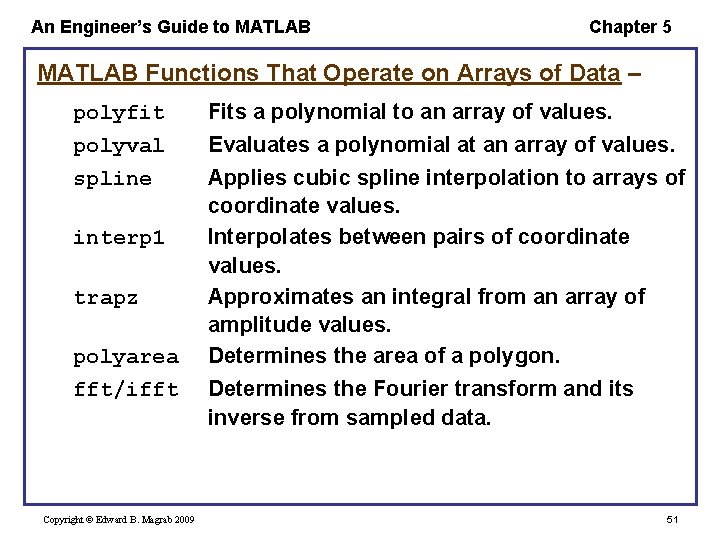
An Engineer’s Guide to MATLAB Chapter 5 MATLAB Functions That Operate on Arrays of Data – polyfit polyval spline interp 1 trapz polyarea fft/ifft Copyright © Edward B. Magrab 2009 Fits a polynomial to an array of values. Evaluates a polynomial at an array of values. Applies cubic spline interpolation to arrays of coordinate values. Interpolates between pairs of coordinate values. Approximates an integral from an array of amplitude values. Determines the area of a polygon. Determines the Fourier transform and its inverse from sampled data. 51

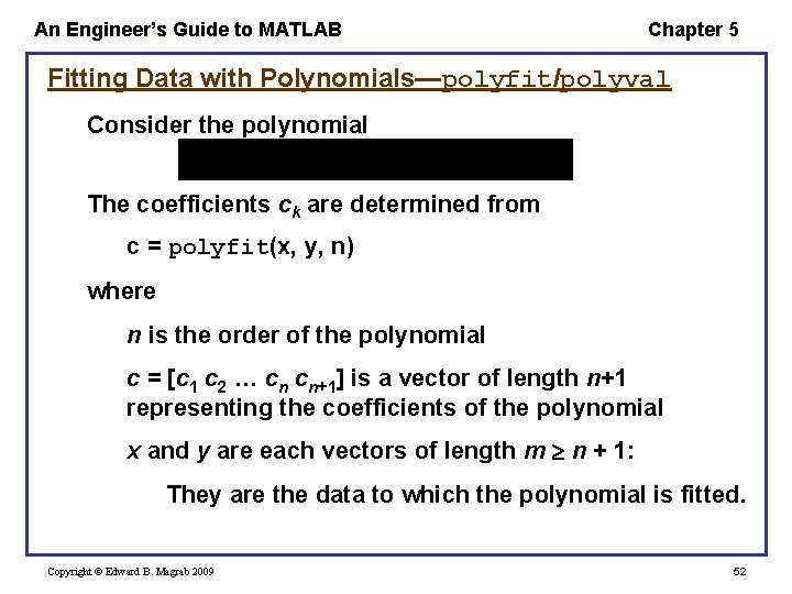
An Engineer’s Guide to MATLAB Chapter 5 Fitting Data with Polynomials—polyfit/polyval Consider the polynomial The coefficients ck are determined from c = polyfit(x, y, n) where n is the order of the polynomial c = [c 1 c 2 … cn cn+1] is a vector of length n+1 representing the coefficients of the polynomial x and y are each vectors of length m n + 1: They are the data to which the polynomial is fitted. Copyright © Edward B. Magrab 2009 52

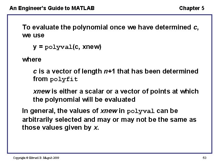
An Engineer’s Guide to MATLAB Chapter 5 To evaluate the polynomial once we have determined c, we use y = polyval(c, xnew) where c is a vector of length n+1 that has been determined from polyfit xnew is either a scalar or a vector of points at which the polynomial will be evaluated In general, the values of xnew in polyval can be arbitrarily selected and may or may not be the same as those values given by x. Copyright © Edward B. Magrab 2009 53

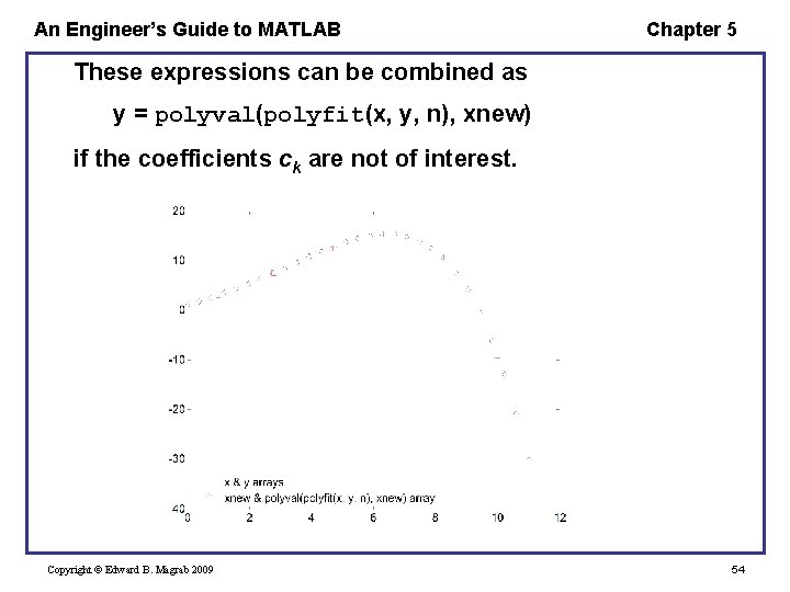
An Engineer’s Guide to MATLAB Chapter 5 These expressions can be combined as y

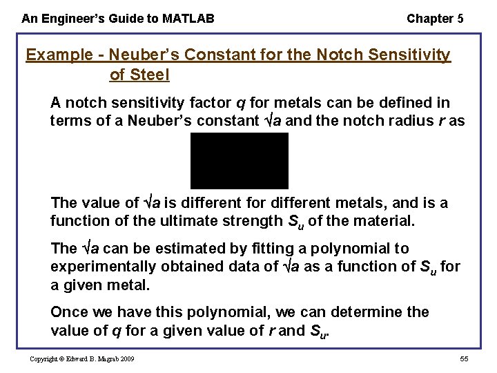
An Engineer’s Guide to MATLAB Chapter 5 Example - Neuber’s Constant for the Notch Sensitivity of Steel A notch sensitivity factor q for metals can be defined in terms of a Neuber’s constant a and the notch radius r as The value of a is different for different metals, and is a function of the ultimate strength Su of the material. The a can be estimated by fitting a polynomial to experimentally obtained data of a as a function of Su for a given metal. Once we have this polynomial, we can determine the value of q for a given value of r and Su. Copyright © Edward B. Magrab 2009 55

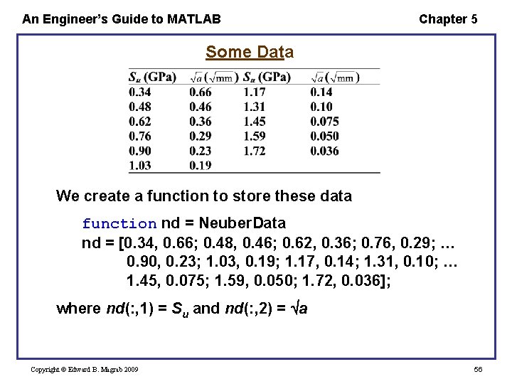
An Engineer’s Guide to MATLAB Chapter 5 Some Data We create a function to store these data function nd = Neuber. Data nd = [0. 34, 0. 66; 0. 48, 0. 46; 0. 62, 0. 36; 0. 76, 0. 29; … 0. 90, 0. 23; 1. 03, 0. 19; 1. 17, 0. 14; 1. 31, 0. 10; … 1. 45, 0. 075; 1. 59, 0. 050; 1. 72, 0. 036]; where nd(: , 1) = Su and nd(: , 2) = a Copyright © Edward B. Magrab 2009 56

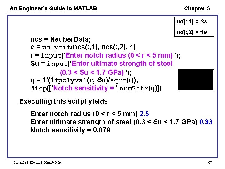
An Engineer’s Guide to MATLAB Chapter 5 nd(: , 1) = Su nd(: , 2) = a ncs = Neuber. Data; c = polyfit(ncs(: , 1), ncs(: , 2), 4); r = input('Enter notch radius (0 < r < 5 mm) '); Su = input('Enter ultimate strength of steel (0. 3 < Su < 1. 7 GPa) '); q = 1/(1+polyval(c, Su)/sqrt(r)); disp(['Notch sensitivity = ' num 2 str(q)]) Executing this script yields Enter notch radius (0 < r < 5 mm) 2. 5 Enter ultimate strength of steel (0. 3 < Su < 1. 7 GPa) 0. 93 Notch sensitivity = 0. 879 Copyright © Edward B. Magrab 2009 57

An Engineer’s Guide to MATLAB Chapter 5 Fitting Data with spline To generate smooth curves that pass through a set of discrete data values we use splines. The function that performs this curve generation is Y = spline(x, y, X) where y is y(x) x and y are vectors of the same length that are used to create the functional relationship y(x) X is a scalar or vector for which the values of Y = y(X) are desired In general, x X. Copyright © Edward B. Magrab 2009 58

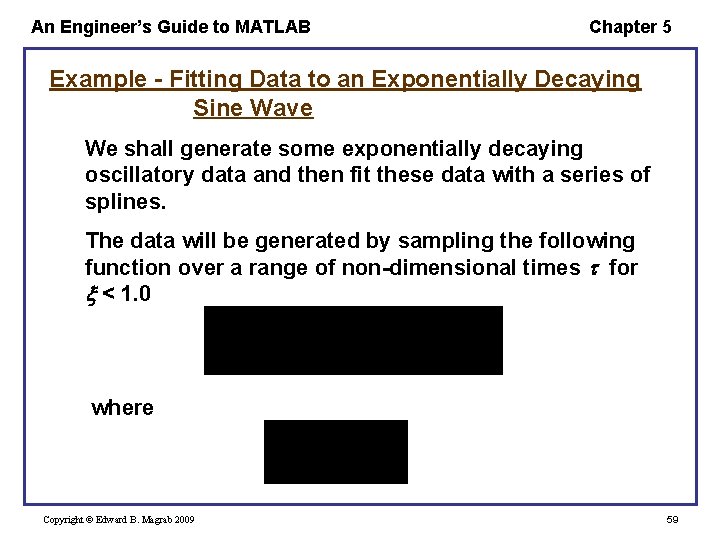
An Engineer’s Guide to MATLAB Chapter 5 Example - Fitting Data to an Exponentially Decaying Sine Wave We shall generate some exponentially decaying oscillatory data and then fit these data with a series of splines. The data will be generated by sampling the following function over a range of non-dimensional times for < 1. 0 where Copyright © Edward B. Magrab 2009 59

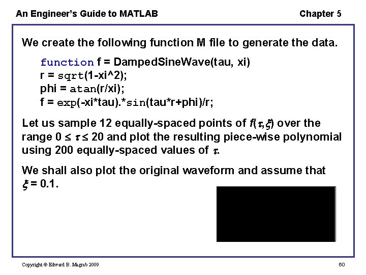
An Engineer’s Guide to MATLAB Chapter 5 We create the following function M file to generate the data. function f = Damped. Sine. Wave(tau, xi) r = sqrt(1 -xi^2); phi = atan(r/xi); f = exp(-xi*tau). *sin(tau*r+phi)/r; Let us sample 12 equally-spaced points of f( , ) over the range 0 20 and plot the resulting piece-wise polynomial using 200 equally-spaced values of . We shall also plot the original waveform and assume that = 0. 1. Copyright © Edward B. Magrab 2009 60

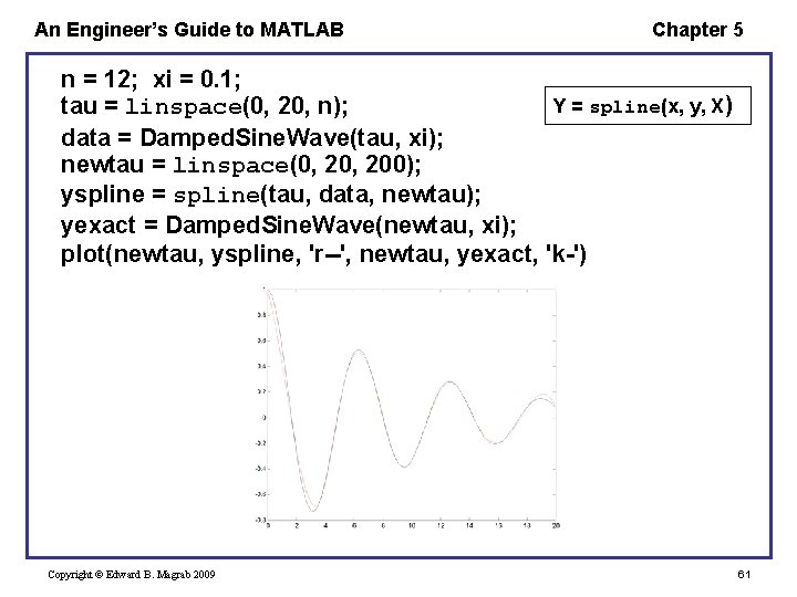
An Engineer’s Guide to MATLAB Chapter 5 n = 12; xi = 0. 1; Y = spline(x, y, X) tau = linspace(0, 20, n); data = Damped. Sine. Wave(tau, xi); newtau = linspace(0, 200); yspline = spline(tau, data, newtau); yexact = Damped. Sine. Wave(newtau, xi); plot(newtau, yspline, 'r--', newtau, yexact, 'k-') Copyright © Edward B. Magrab 2009 61

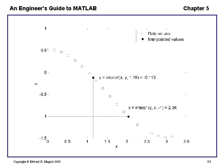
An Engineer’s Guide to MATLAB Chapter 5 Interpolation of Data—interp 1 To approximate the location of a value that lies between a pair of data points, we must interpolate. The function that does this interpolation is V = interp 1(u, v, U) where the array V will have the same length as U, v is v(u) u and v are vectors of the same length U is a scalar or vector of values for u for which V desired In general, u U. Copyright © Edward B. Magrab 2009 62

An Engineer’s Guide to MATLAB Copyright © Edward B. Magrab 2009 Chapter 5 63

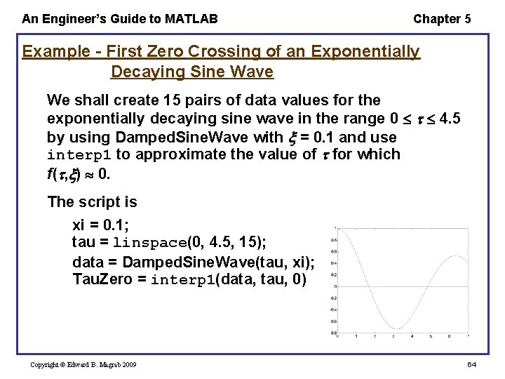
An Engineer’s Guide to MATLAB Chapter 5 Example - First Zero Crossing of an Exponentially Decaying Sine Wave We shall create 15 pairs of data values for the exponentially decaying sine wave in the range 0 4. 5 by using Damped. Sine. Wave with = 0. 1 and use interp 1 to approximate the value of for which f( , ) 0. The script is xi = 0. 1; tau = linspace(0, 4. 5, 15); data = Damped. Sine. Wave(tau, xi); Tau. Zero = interp 1(data, tau, 0) Copyright © Edward B. Magrab 2009 64

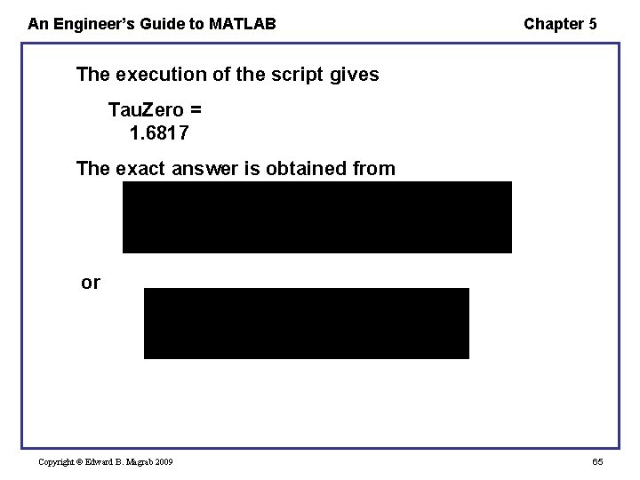
An Engineer’s Guide to MATLAB Chapter 5 The execution of the script gives Tau.

An Engineer’s Guide to MATLAB Chapter 5 Numerical Integration—trapz One can obtain an approximation to a single integral using trapz, whose form is Area = trapz(x, y) where x and the corresponding values of y are arrays The function performs the summation of the product of the average of adjacent y values and the corresponding x interval separating them. Copyright © Edward B. Magrab 2009 66

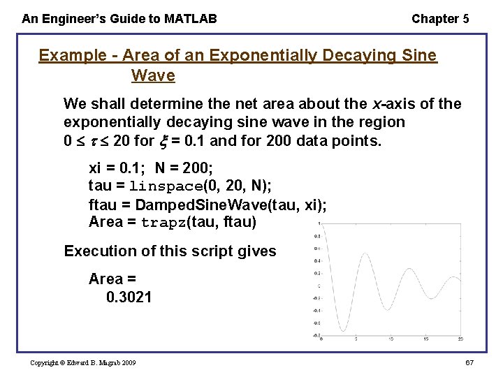
An Engineer’s Guide to MATLAB Chapter 5 Example - Area of an Exponentially Decaying Sine Wave We shall determine the net area about the x-axis of the exponentially decaying sine wave in the region 0 20 for = 0. 1 and for 200 data points. xi = 0. 1; N = 200; tau = linspace(0, 20, N); ftau = Damped. Sine. Wave(tau, xi); Area = trapz(tau, ftau) Execution of this script gives Area = 0. 3021 Copyright © Edward B. Magrab 2009 67

An Engineer’s Guide to MATLAB Chapter 5 Example continued – To determine the area of the positive and negative portions of the waveform, we use logical functions to isolate the negative and positive portions of the waveform as follows. xi = 0. 1; tau = linspace(0, 200); ftau = Damped. Sine. Wave(tau, xi); Logicp = (ftau >= 0); Pos. Area = trapz(tau, ftau. *Logicp); Logicn = (ftau < 0); Neg. Area = trapz(tau, ftau. *Logicn); disp(['Positive area = ' num 2 str(Pos. Area)]) disp(['Negative area = ' num 2 str(Neg. Area)]) disp([['Net area = ' num 2 str(Pos. Area+Neg. Area)]]) Copyright © Edward B. Magrab 2009 68

An Engineer’s Guide to MATLAB Chapter 5 Upon execution, we obtain Positive area =

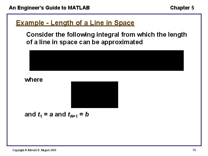
An Engineer’s Guide to MATLAB Chapter 5 Example - Length of a Line in Space Consider the following integral from which the length of a line in space can be approximated where and t 1 = a and t. N+1 = b Copyright © Edward B. Magrab 2009 70

An Engineer’s Guide to MATLAB Chapter 5 We shall employ the function diff which computes the difference between successive elements of a vector; that is, for a vector x = [x 1 x 2 … xn] diff creates a vector q with n 1 elements of the form q = [x 2 x 1, x 3 x 2, … , xn xn-1] For a vector x, diff is simply q = x(2: end)-x(1: end-1); Copyright © Edward B. Magrab 2009 71

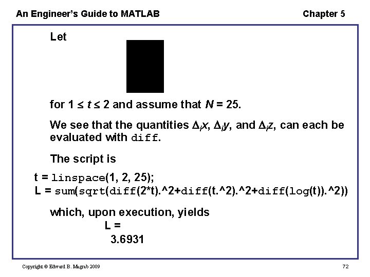
An Engineer’s Guide to MATLAB Chapter 5 Let for 1 t 2 and assume that N = 25. We see that the quantities ix, iy, and iz, can each be evaluated with diff. The script is t = linspace(1, 2, 25); L = sum(sqrt(diff(2*t). ^2+diff(t. ^2). ^2+diff(log(t)). ^2)) which, upon execution, yields L= 3. 6931 Copyright © Edward B. Magrab 2009 72

An Engineer’s Guide to MATLAB Chapter 5 Area of a Polygon—polyarea One can obtain the area of an n-sided polygon, where each side of the polygon is represented by its end points, with the use of polyarea(x, y) where x and y are vectors of the same length that contain the (x, y) coordinates of the endpoints of each side of the polygon. Each (x, y) coordinate pair is the end point of two adjacent sides of the polygon; hence, for an n-sided polygon, we need n + 1 pairs of end points. Copyright © Edward B. Magrab 2009 73

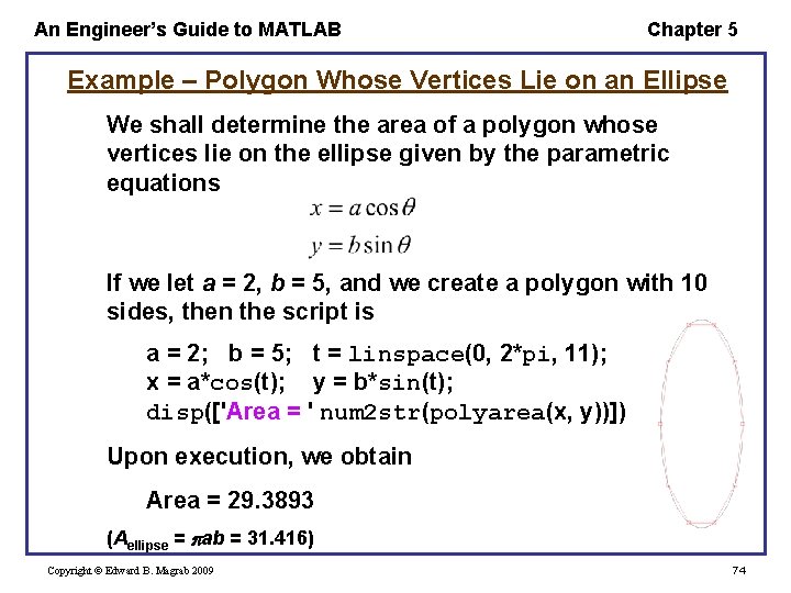
An Engineer’s Guide to MATLAB Chapter 5 Example – Polygon Whose Vertices Lie on an Ellipse We shall determine the area of a polygon whose vertices lie on the ellipse given by the parametric equations If we let a = 2, b = 5, and we create a polygon with 10 sides, then the script is a = 2; b = 5; t = linspace(0, 2*pi, 11); x = a*cos(t); y = b*sin(t); disp(['Area = ' num 2 str(polyarea(x, y))]) Upon execution, we obtain Area = 29. 3893 (Aellipse = ab = 31. 416) Copyright © Edward B. Magrab 2009 74

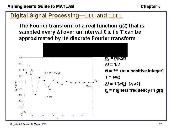
An Engineer’s Guide to MATLAB Chapter 5 Digital Signal Processing—fft and ifft The Fourier transform of a real function g(t) that is sampled every t over an interval 0 t T can be approximated by its discrete Fourier transform gk = g(k t) f = 1/T N = 2 m (m = positive integer) T = N t t = 1/( fh) ( >2) fh = highest frequency in g(t) Copyright © Edward B. Magrab 2009 75

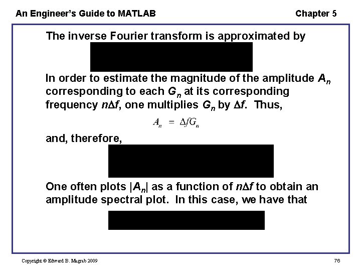
An Engineer’s Guide to MATLAB Chapter 5 The inverse Fourier transform is approximated by In order to estimate the magnitude of the amplitude An corresponding to each Gn at its corresponding frequency n f, one multiplies Gn by f. Thus, and, therefore, One often plots |An| as a function of n f to obtain an amplitude spectral plot. In this case, we have that Copyright © Edward B. Magrab 2009 76

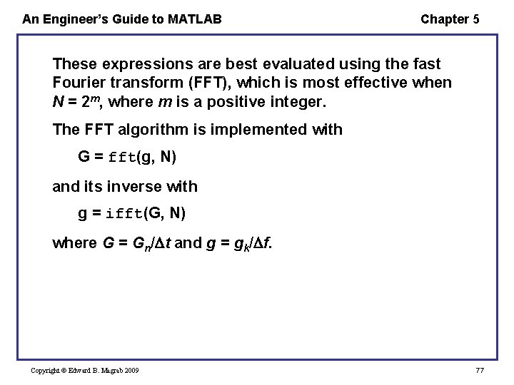
An Engineer’s Guide to MATLAB Chapter 5 These expressions are best evaluated using the fast Fourier transform (FFT), which is most effective when N = 2 m, where m is a positive integer. The FFT algorithm is implemented with G = fft(g, N) and its inverse with g = ifft(G, N) where G = Gn/ t and g = gk/ f. Copyright © Edward B. Magrab 2009 77

An Engineer’s Guide to MATLAB Chapter 5 Example - Fourier Transform of a Sine Wave Let us determine an amplitude spectral plot of a sampled sine wave of duration T under the following conditions. and We assume that Bo = 2. 5, fo = 10 Hz, K = 5, and m = 10 (N = 1024). The script is Copyright © Edward B. Magrab 2009 78

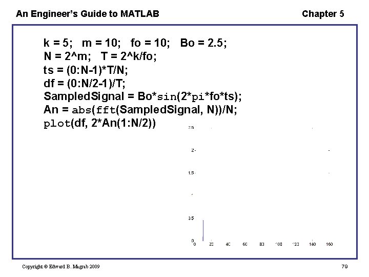
An Engineer’s Guide to MATLAB Chapter 5 k = 5; m = 10; fo = 10; Bo = 2. 5; N = 2^m; T = 2^k/fo; ts = (0: N-1)*T/N; df = (0: N/2 -1)/T; Sampled. Signal = Bo*sin(2*pi*fo*ts); An = abs(fft(Sampled. Signal, N))/N; plot(df, 2*An(1: N/2)) Copyright © Edward B. Magrab 2009 79

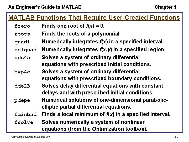
An Engineer’s Guide to MATLAB Chapter 5 MATLAB Functions That Require User-Created Functions fzero roots quadl dblquad Finds one root of f(x) = 0. Finds the roots of a polynomial Numerically integrates f(x) in a specified interval. Numerically integrates f(x, y) in a specified region. Solves a system of ordinary differential equations with prescribed initial conditions. bvp 4 c Solves a system of ordinary differential equations with prescribed boundary conditions. dde 23 Solves delay differential equations with constant delays and with prescribed initial conditions. pdepe Numerical solutions of one-dimensional parabolicelliptic partial differential equations. fminbnd Finds a local minimum of f(x) in a specified interval. fsolve Solves numerically a system of nonlinear equations (from the Optimization toolbox). ode 45 Copyright © Edward B. Magrab 2009 80

An Engineer’s Guide to MATLAB Chapter 5 Zeros of Functions—fzero and roots/poly fzero The are many equations for which an explicit algebraic solution to f(x) = 0 cannot be found. In these cases, one uses fzero to find numerically one solution to the real function f(x) = 0 within a tolerance to in either the neighborhood of xo or within the range [x 1, x 2]. The function can also transfer pj, j = 1, 2, …, parameters to the function defining f(x). Copyright © Edward B. Magrab 2009 81

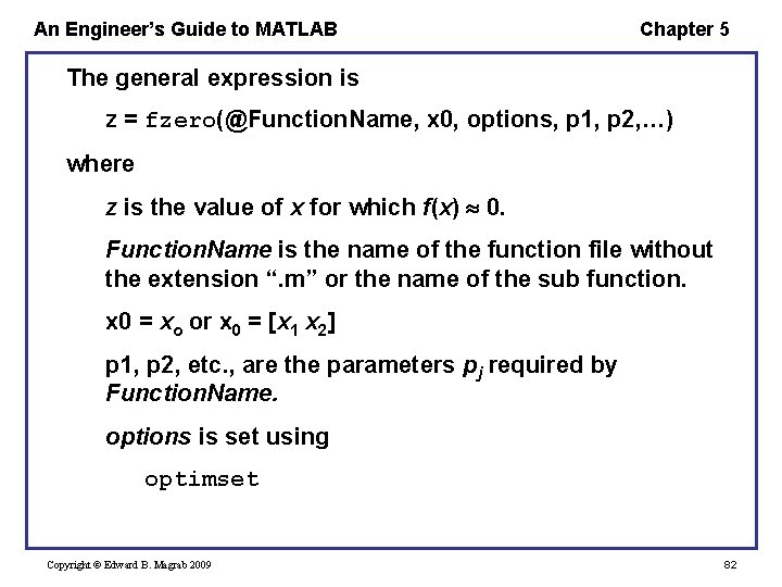
An Engineer’s Guide to MATLAB Chapter 5 The general expression is z = fzero(@Function. Name, x 0, options, p 1, p 2, …) where z is the value of x for which f(x) 0. Function. Name is the name of the function file without the extension “. m” or the name of the sub function. x 0 = xo or x 0 = [x 1 x 2] p 1, p 2, etc. , are the parameters pj required by Function. Name. options is set using optimset Copyright © Edward B. Magrab 2009 82

An Engineer’s Guide to MATLAB Chapter 5 The function optimset is a general parameter-adjusting function that is used by several MATLAB functions, primarily from the Optimization toolbox. Copyright © Edward B. Magrab 2009 83

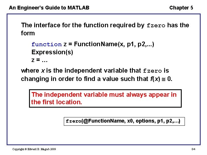
An Engineer’s Guide to MATLAB Chapter 5 The interface for the function required by fzero has the form function z = Function. Name(x, p 1, p 2, . . . ) Expression(s) z=… where x is the independent variable that fzero is changing in order to find a value such that f(x) 0. The independent variable must always appear in the first location. fzero(@Function. Name, x 0, options, p 1, p 2, …) Copyright © Edward B. Magrab 2009 84

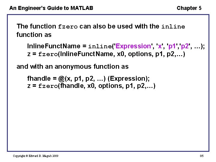
An Engineer’s Guide to MATLAB Chapter 5 The function fzero can also be used with the inline function as Inline. Funct. Name = inline('Expression', 'x', 'p 1', 'p 2', …); z = fzero(Inline. Funct. Name, x 0, options, p 1, p 2, …) and with an anonymous function as fhandle = @(x, p 1, p 2, …) (Expression); z = fzero(fhandle, x 0, options, p 1, p 2, …) Copyright © Edward B. Magrab 2009 85

An Engineer’s Guide to MATLAB Chapter 5 Warning – Care must be exercised when using fzero with some of MATLAB’s functions Let us determine the root of J 1(x) = 0 near 3, where J 1(x) is the Bessel function of the first kind of order 1. The Bessel function is a oscillatory function similar to trigonometric functions. The Bessel function is obtained from besselj(n, x) where n is the order (= 1 in this case) and x is the independent variable. Copyright © Edward B. Magrab 2009 86

An Engineer’s Guide to MATLAB Chapter 5 We cannot use this function directly because the independent variable x is not the first variable in the function, n is. Hence, we create a new function using inline as follows besseljx = inline('besselj(n, x)', 'x', 'n'); a = fzero(besseljx, 3, [], 1) Upon execution, we obtain a= 3. 8317 Notice that in order to transfer the parameter p 1 = n = 1 to the function besseljx, we had to place a value of 1 in the fourth location of fzero. Copyright © Edward B. Magrab 2009 87

An Engineer’s Guide to MATLAB Chapter 5 If we were to use an anonymous

An Engineer’s Guide to MATLAB Chapter 5 Extension: Finding Multiple Zeros of a Function – For multi-valued functions whose properties are not known a priori, one could use the following method as one way to determine the search regions for fzero automatically. This method determines the approximate locations of the change in signs in f(x) in a given range of x, and thereby obtains the regions [x 1, x 2] for which fzero conducts its search. This method is presented as an M-file so that it may be used with an arbitrary f(x). Copyright © Edward B. Magrab 2009 89

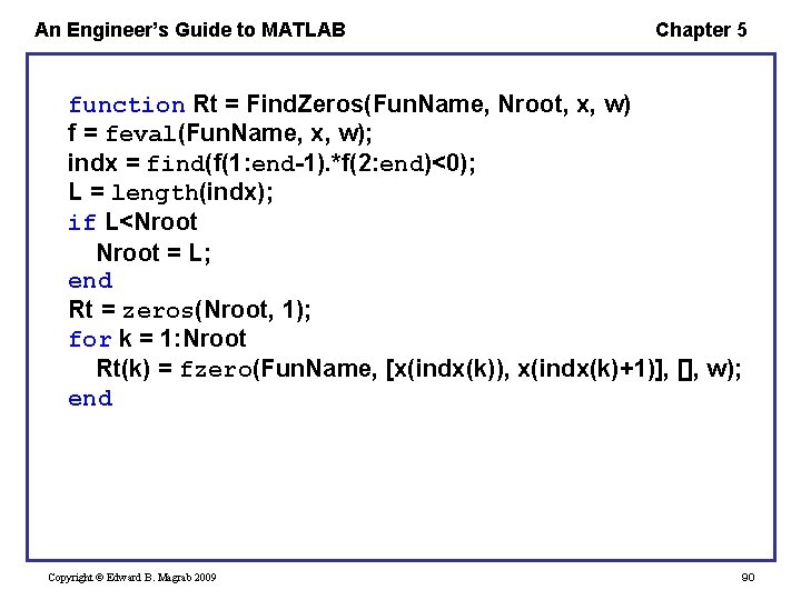
An Engineer’s Guide to MATLAB Chapter 5 function Rt = Find. Zeros(Fun. Name, Nroot, x, w) f = feval(Fun. Name, x, w); indx = find(f(1: end-1). *f(2: end)<0); L = length(indx); if L<Nroot = L; end Rt = zeros(Nroot, 1); for k = 1: Nroot Rt(k) = fzero(Fun. Name, [x(indx(k)), x(indx(k)+1)], [], w); end Copyright © Edward B. Magrab 2009 90

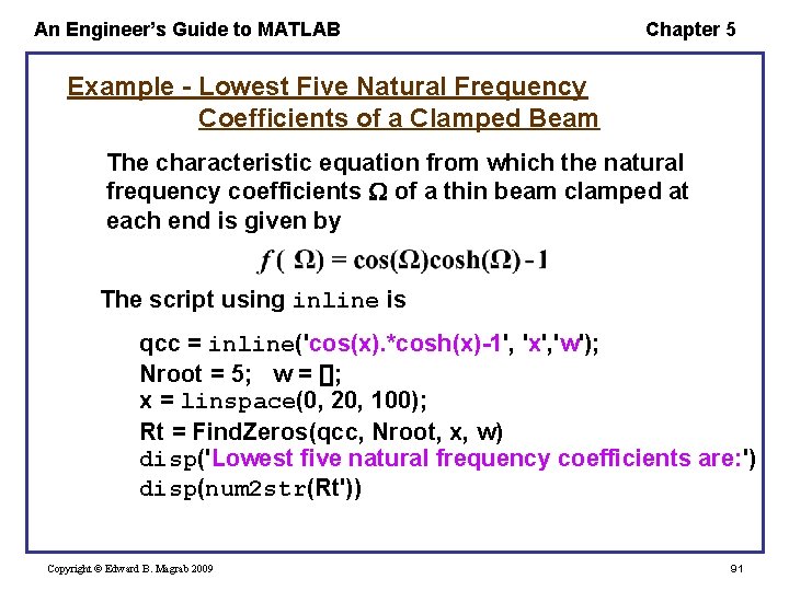
An Engineer’s Guide to MATLAB Chapter 5 Example - Lowest Five Natural Frequency Coefficients of a Clamped Beam The characteristic equation from which the natural frequency coefficients of a thin beam clamped at each end is given by The script using inline is qcc = inline('cos(x). *cosh(x)-1', 'x', 'w'); Nroot = 5; w = []; x = linspace(0, 20, 100); Rt = Find. Zeros(qcc, Nroot, x, w) disp('Lowest five natural frequency coefficients are: ') disp(num 2 str(Rt')) Copyright © Edward B. Magrab 2009 91

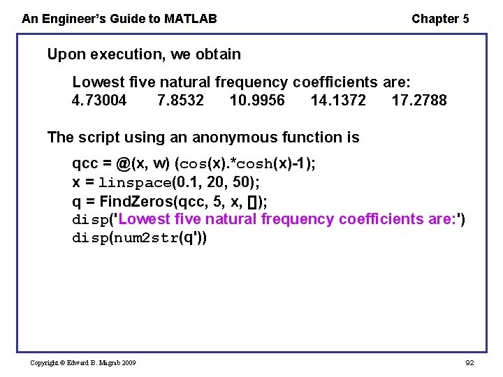
An Engineer’s Guide to MATLAB Chapter 5 Upon execution, we obtain Lowest five natural frequency coefficients are: 4. 73004 7. 8532 10. 9956 14. 1372 17. 2788 The script using an anonymous function is qcc = @(x, w) (cos(x). *cosh(x)-1); x = linspace(0. 1, 20, 50); q = Find. Zeros(qcc, 5, x, []); disp('Lowest five natural frequency coefficients are: ') disp(num 2 str(q')) Copyright © Edward B. Magrab 2009 92

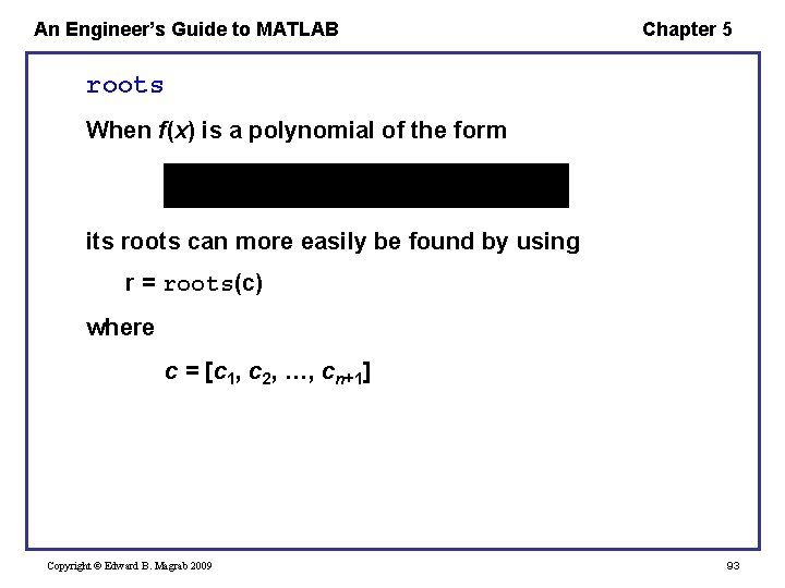
An Engineer’s Guide to MATLAB Chapter 5 roots When f(x) is a polynomial of the form its roots can more easily be found by using r = roots(c) where c = [c 1, c 2, …, cn+1] Copyright © Edward B. Magrab 2009 93

An Engineer’s Guide to MATLAB Chapter 5 poly The inverse of roots is c = poly(r) which returns c, the polynomial’s coefficients, and r is a vector of roots. In the general case, r is a vector of real and/or complex numbers. Copyright © Edward B. Magrab 2009 94

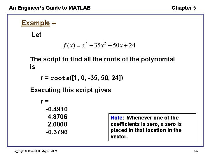
An Engineer’s Guide to MATLAB Chapter 5 Example – Let The script to find all the roots of the polynomial is r = roots([1, 0, -35, 50, 24]) Executing this script gives r= -6. 4910 4. 8706 2. 0000 -0. 3796 Copyright © Edward B. Magrab 2009 Note: Whenever one of the coefficients is zero, a zero is placed in that location in the vector. 95

An Engineer’s Guide to MATLAB Chapter 5 Notice that the roots do not come out in any particular order. To order them, one uses sort. Thus, r = sort(roots([1, 0, -35, 50, 24])) which, upon execution, gives r= -6. 4910 -0. 3796 2. 0000 4. 8706 Copyright © Edward B. Magrab 2009 96

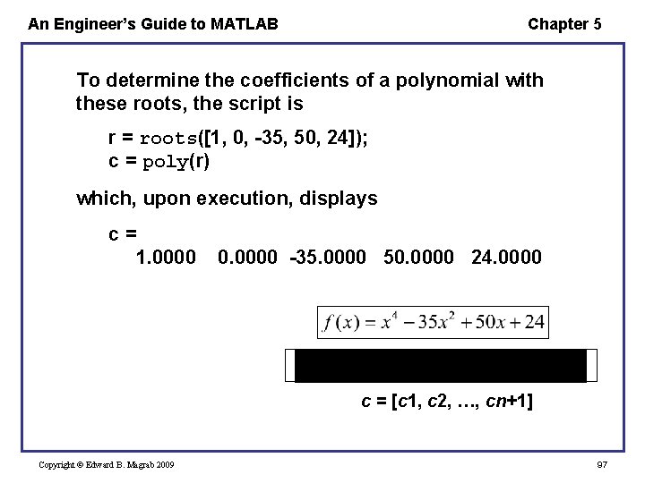
An Engineer’s Guide to MATLAB Chapter 5 To determine the coefficients of a polynomial with these roots, the script is r = roots([1, 0, -35, 50, 24]); c = poly(r) which, upon execution, displays c= 1. 0000 0. 0000 -35. 0000 50. 0000 24. 0000 c = [c 1, c 2, …, cn+1] Copyright © Edward B. Magrab 2009 97

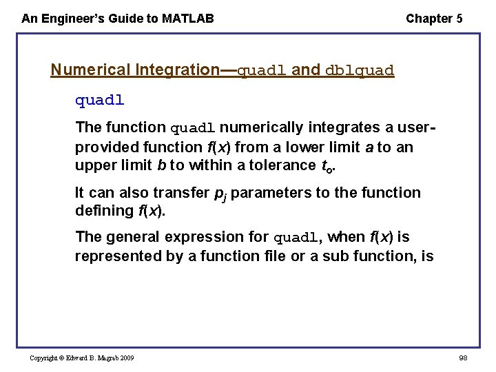
An Engineer’s Guide to MATLAB Chapter 5 Numerical Integration—quadl and dblquadl The function quadl numerically integrates a userprovided function f(x) from a lower limit a to an upper limit b to within a tolerance to. It can also transfer pj parameters to the function defining f(x). The general expression for quadl, when f(x) is represented by a function file or a sub function, is Copyright © Edward B. Magrab 2009 98

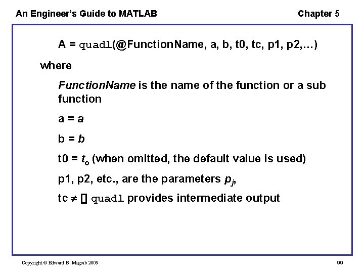
An Engineer’s Guide to MATLAB Chapter 5 A = quadl(@Function. Name, a, b, t 0, tc, p 1, p 2, …) where Function. Name is the name of the function or a sub function a=a b=b t 0 = to (when omitted, the default value is used) p 1, p 2, etc. , are the parameters pj, tc [] quadl provides intermediate output Copyright © Edward B. Magrab 2009 99

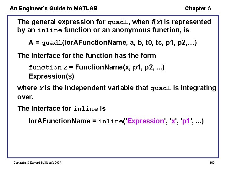
An Engineer’s Guide to MATLAB Chapter 5 The general expression for quadl, when f(x) is represented by an inline function or an anonymous function, is A = quadl(Ior. AFunction. Name, a, b, t 0, tc, p 1, p 2, …) The interface for the function has the form function z = Function. Name(x, p 1, p 2, . . . ) Expression(s) where x is the independent variable that quadl is integrating over. The interface for inline is Ior. AFunction. Name = inline('Expression', 'x', 'p 1', . . . ) Copyright © Edward B. Magrab 2009 100

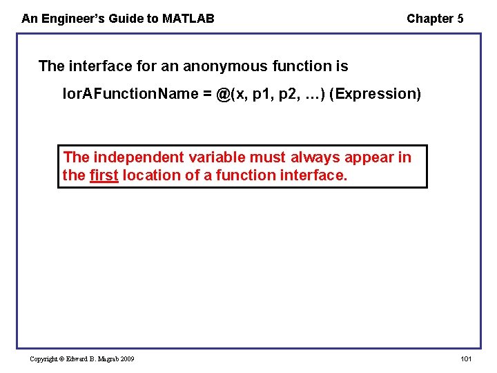
An Engineer’s Guide to MATLAB Chapter 5 The interface for an anonymous function is Ior. AFunction. Name = @(x, p 1, p 2, …) (Expression) The independent variable must always appear in the first location of a function interface. Copyright © Edward B. Magrab 2009 101

An Engineer’s Guide to MATLAB Chapter 5 Example – Area of an Exponentially Decaying Sine Wave Revisited The damped sine wave is represented by the function Damped. Sine. Wave. If we again let = 0. 1 and integrate from 0 20, then the script is xi = 0. 1; Area = quadl(@Damped. Sine. Wave, 0, 20, [], xi) Upon execution, we obtain Area = 0. 3022 From trapz – Area = 0. 3021 Copyright © Edward B. Magrab 2009 A = quadl(@Function. Name, a, b, t 0, tc, p 1, p 2, …) 102

An Engineer’s Guide to MATLAB Chapter 5 dblquad The function dblquad numerically integrates a userprovided function f(x, y) from a lower limit xl to an upper limit xu in the x-direction and from a lower limit yl to an upper limit yu in the y-direction to within a tolerance to. It can also transfer pj parameters to the function defining f(x, y). Copyright © Edward B. Magrab 2009 103

An Engineer’s Guide to MATLAB Chapter 5 The general expression for dblquad, when f(x, y) is represented by a function or a sub function, is dblquad(@Function. Name, xl, xu, yl, yu, t 0, meth, p 1, p 2, …) where Function. Name is the name of the function or sub function xl = xl xu = xu yl = yl yu = yu t 0 = to (when omitted, the default value is used) p 1, p 2, etc. , are the parameters pj when meth = [], quadl is the method used Copyright © Edward B. Magrab 2009 104

An Engineer’s Guide to MATLAB Chapter 5 When the function is created by inline or an anonymous function, then dblquad(Ior. AFunction. Name, xl, xu, yl, yu, t 0, meth, p 1, p 2, …) where Ior. AFunction. Name is the name of the inline function or anonymous function The interface for the function file has the form function z = Function. Name(x, y, p 1, p 2, . . . ) Expression(s) z=… Copyright © Edward B. Magrab 2009 105

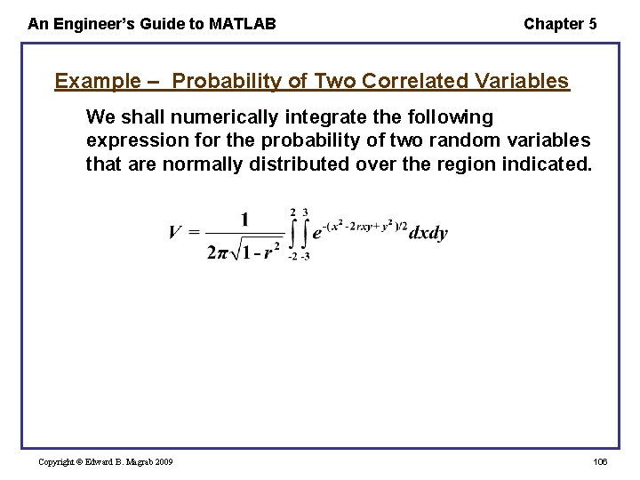
An Engineer’s Guide to MATLAB Chapter 5 Example – Probability of Two Correlated Variables We shall numerically integrate the following expression for the probability of two random variables that are normally distributed over the region indicated. Copyright © Edward B. Magrab 2009 106

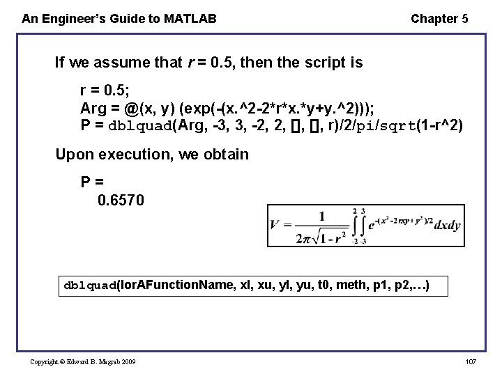
An Engineer’s Guide to MATLAB Chapter 5 If we assume that r = 0. 5, then the script is r = 0. 5; Arg = @(x, y) (exp(-(x. ^2 -2*r*x. *y+y. ^2))); P = dblquad(Arg, -3, 3, -2, 2, [], r)/2/pi/sqrt(1 -r^2) Upon execution, we obtain P= 0. 6570 dblquad(Ior. AFunction. Name, xl, xu, yl, yu, t 0, meth, p 1, p 2, …) Copyright © Edward B. Magrab 2009 107

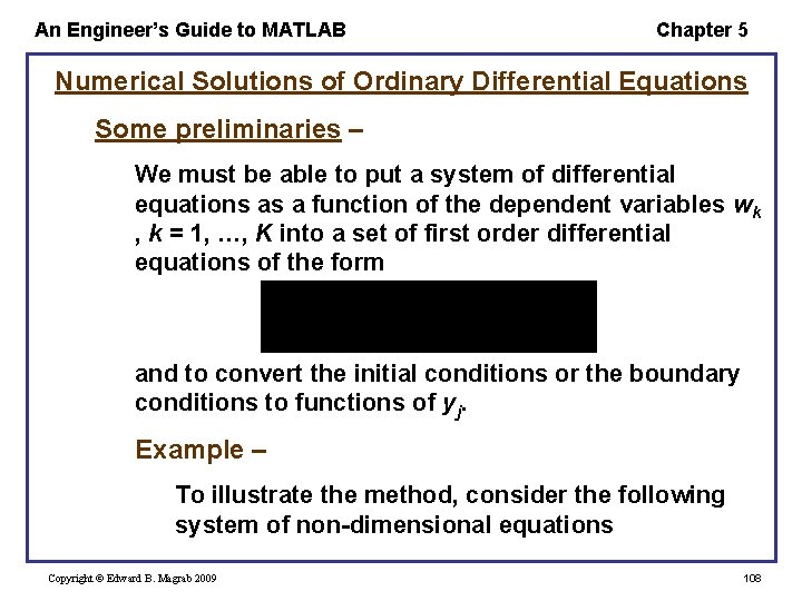
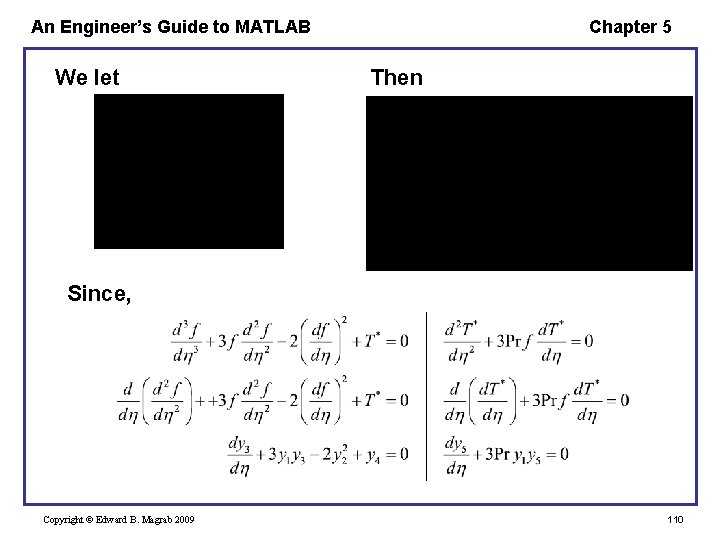
An Engineer’s Guide to MATLAB Chapter 5 Numerical Solutions of Ordinary Differential Equations Some preliminaries – We must be able to put a system of differential equations as a function of the dependent variables wk , k = 1, …, K into a set of first order differential equations of the form and to convert the initial conditions or the boundary conditions to functions of yj. Example – To illustrate the method, consider the following system of non-dimensional equations Copyright © Edward B. Magrab 2009 108

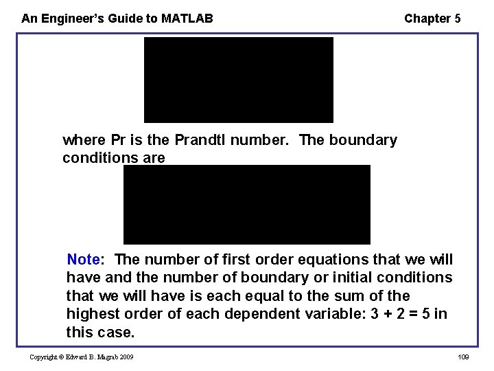
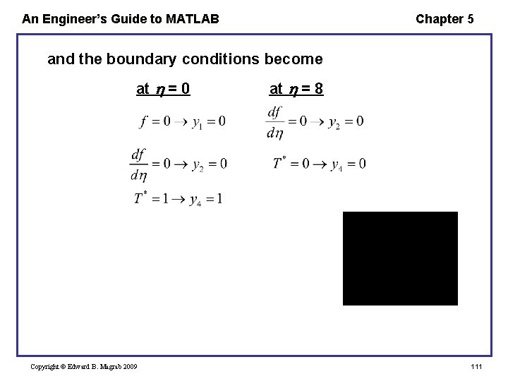
An Engineer’s Guide to MATLAB Chapter 5 where Pr is the Prandtl number. The boundary conditions are Note: The number of first order equations that we will have and the number of boundary or initial conditions that we will have is each equal to the sum of the highest order of each dependent variable: 3 + 2 = 5 in this case. Copyright © Edward B. Magrab 2009 109

An Engineer’s Guide to MATLAB We let Chapter 5 Then Since, Copyright © Edward

An Engineer’s Guide to MATLAB Chapter 5 and the boundary conditions become at =

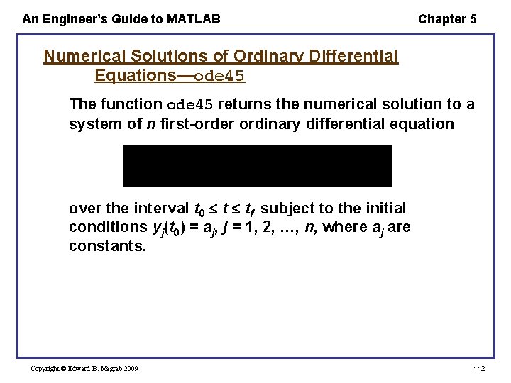
An Engineer’s Guide to MATLAB Chapter 5 Numerical Solutions of Ordinary Differential Equations—ode 45 The function ode 45 returns the numerical solution to a system of n first-order ordinary differential equation over the interval t 0 t tf subject to the initial conditions yj(t 0) = aj, j = 1, 2, …, n, where aj are constants. Copyright © Edward B. Magrab 2009 112

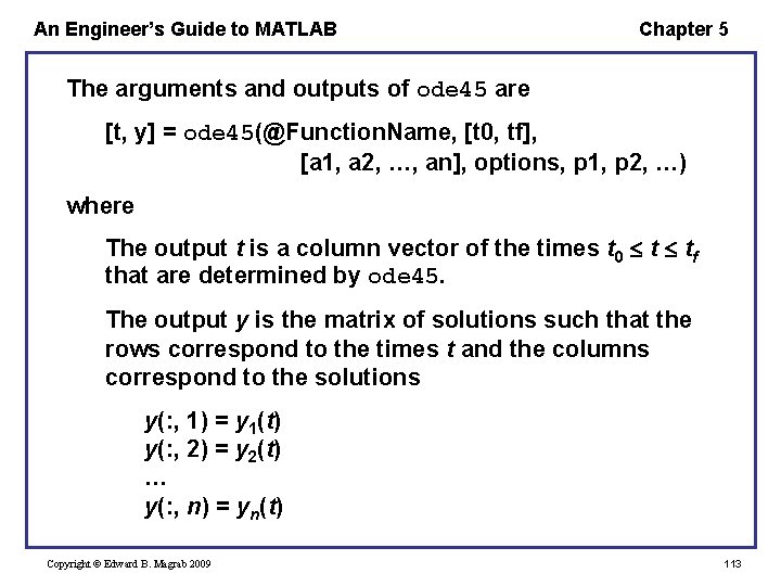
An Engineer’s Guide to MATLAB Chapter 5 The arguments and outputs of ode 45 are [t, y] = ode 45(@Function. Name, [t 0, tf], [a 1, a 2, …, an], options, p 1, p 2, …) where The output t is a column vector of the times t 0 t tf that are determined by ode 45. The output y is the matrix of solutions such that the rows correspond to the times t and the columns correspond to the solutions y(: , 1) = y 1(t) y(: , 2) = y 2(t) … y(: , n) = yn(t) Copyright © Edward B. Magrab 2009 113

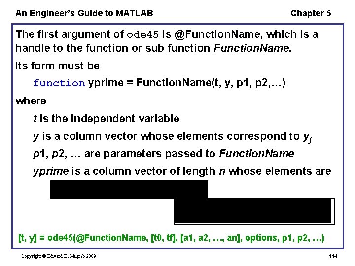
An Engineer’s Guide to MATLAB Chapter 5 The first argument of ode 45 is @Function. Name, which is a handle to the function or sub function Function. Name. Its form must be function yprime = Function. Name(t, y, p 1, p 2, …) where t is the independent variable y is a column vector whose elements correspond to yj p 1, p 2, … are parameters passed to Function. Name yprime is a column vector of length n whose elements are [t, y] = ode 45(@Function. Name, [t 0, tf], [a 1, a 2, …, an], options, p 1, p 2, …) Copyright © Edward B. Magrab 2009 114

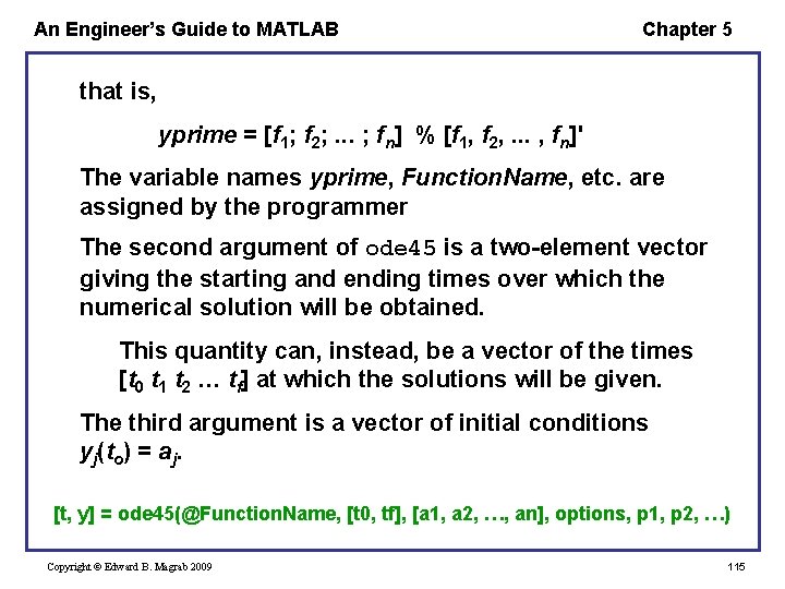
An Engineer’s Guide to MATLAB Chapter 5 that is, yprime = [f 1; f 2; . . . ; fn] % [f 1, f 2, . . . , fn]' The variable names yprime, Function. Name, etc. are assigned by the programmer The second argument of ode 45 is a two-element vector giving the starting and ending times over which the numerical solution will be obtained. This quantity can, instead, be a vector of the times [t 0 t 1 t 2 … tf] at which the solutions will be given. The third argument is a vector of initial conditions yj(to) = aj. [t, y] = ode 45(@Function. Name, [t 0, tf], [a 1, a 2, …, an], options, p 1, p 2, …) Copyright © Edward B. Magrab 2009 115

An Engineer’s Guide to MATLAB Chapter 5 The fourth argument, options, is usually set to null ([]). If some of the solution method tolerances are to be changed, one does this with odeset (see the odeset Help file). The remaining arguments are those that are passed to Function. Name. [t, y] = ode 45(@Function. Name, [t 0, tf], [a 1, a 2, …, an], options, p 1, p 2, …) Copyright © Edward B. Magrab 2009 116

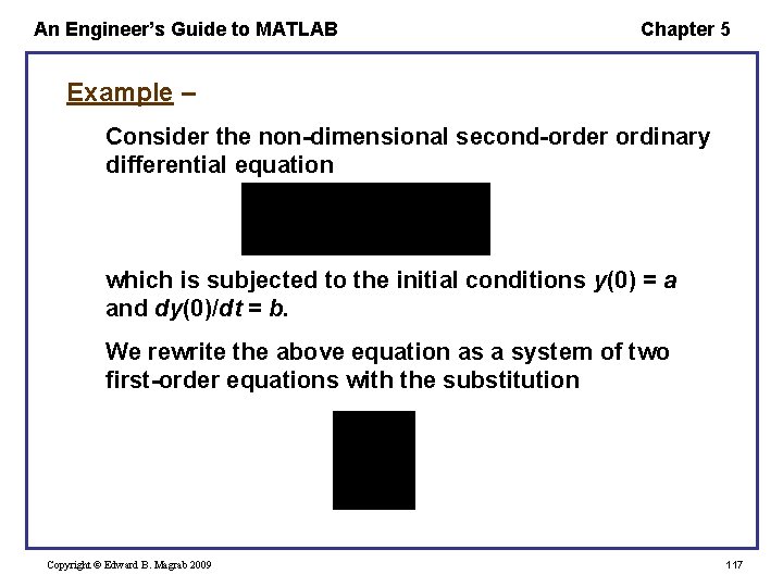
An Engineer’s Guide to MATLAB Chapter 5 Example – Consider the non-dimensional second-order ordinary differential equation which is subjected to the initial conditions y(0) = a and dy(0)/dt = b. We rewrite the above equation as a system of two first-order equations with the substitution Copyright © Edward B. Magrab 2009 117

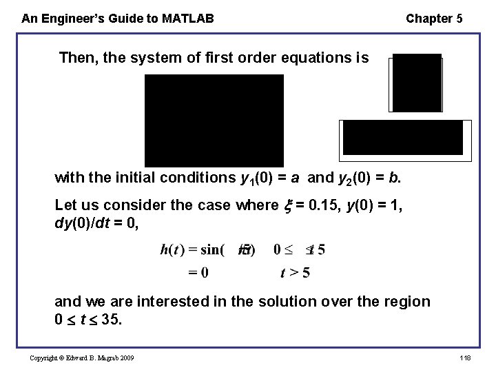
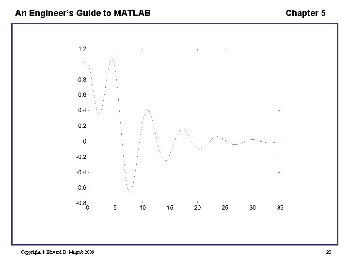
An Engineer’s Guide to MATLAB Chapter 5 Then, the system of first order equations is with the initial conditions y 1(0) = a and y 2(0) = b. Let us consider the case where = 0. 15, y(0) = 1, dy(0)/dt = 0, and we are interested in the solution over the region 0 t 35. Copyright © Edward B. Magrab 2009 118

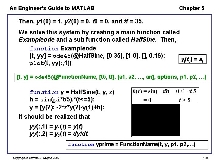
An Engineer’s Guide to MATLAB Chapter 5 Then, y 1(0) = 1, y 2(0) = 0, t 0 = 0, and tf = 35. We solve this system by creating a main function called Exampleode and a sub function called Half. Sine. Then, function Exampleode [t, yy] = ode 45(@Half. Sine, [0 35], [1 0], [], 0. 15); yj(t 0) = aj plot(t, yy(: , 1)) [t, y] = ode 45(@Function. Name, [t 0, tf], [a 1, a 2, …, an], options, p 1, p 2, …) function y = Half. Sine(t, y, z) h = sin(pi*t/5). *(t<=5); y = [y(2); -2*z*y(2)-y(1)+h]; It should be realized that yy(: , 1) = y 1(t) = y(t) yy(: , 2) = y 2(t) = dy/dt function yprime = Function. Name(t, y, p 1, p 2, …) Copyright © Edward B. Magrab 2009 119

An Engineer’s Guide to MATLAB Copyright © Edward B. Magrab 2009 Chapter 5 120

An Engineer’s Guide to MATLAB Chapter 5 Numerical Solutions of Ordinary Differential Equations—bvp 4 c The function bvp 4 c obtains numerical solutions to the two-point boundary value problem. Unlike ode 45, bvp 4 c requires the use of several additional MATLAB functions that were specifically created: bvpinit – initializing function deval – output smoothing function for plotting Several additional user function files must be created. Copyright © Edward B. Magrab 2009 121

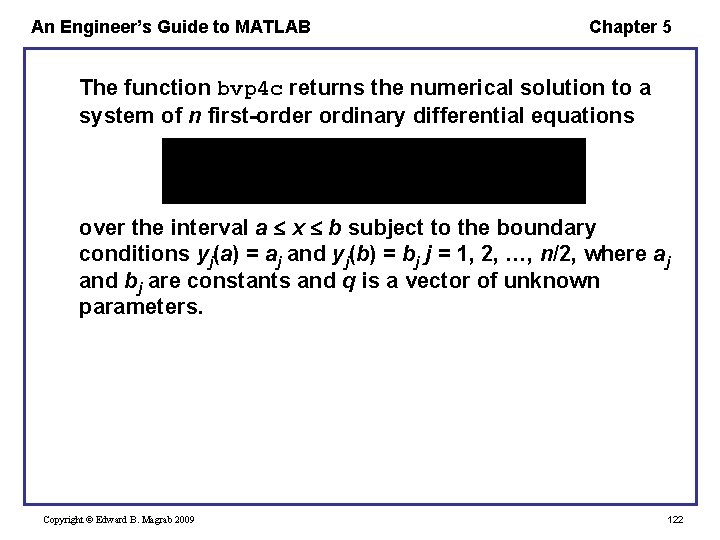
An Engineer’s Guide to MATLAB Chapter 5 The function bvp 4 c returns the numerical solution to a system of n first-order ordinary differential equations over the interval a x b subject to the boundary conditions yj(a) = aj and yj(b) = bj j = 1, 2, …, n/2, where aj and bj are constants and q is a vector of unknown parameters. Copyright © Edward B. Magrab 2009 122

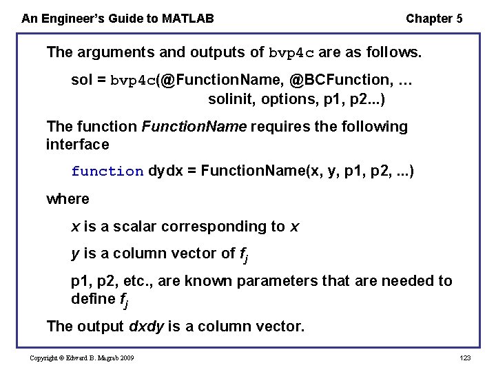
An Engineer’s Guide to MATLAB Chapter 5 The arguments and outputs of bvp 4 c are as follows. sol = bvp 4 c(@Function. Name, @BCFunction, … solinit, options, p 1, p 2. . . ) The function Function. Name requires the following interface function dydx = Function. Name(x, y, p 1, p 2, . . . ) where x is a scalar corresponding to x y is a column vector of fj p 1, p 2, etc. , are known parameters that are needed to define fj The output dxdy is a column vector. Copyright © Edward B. Magrab 2009 123

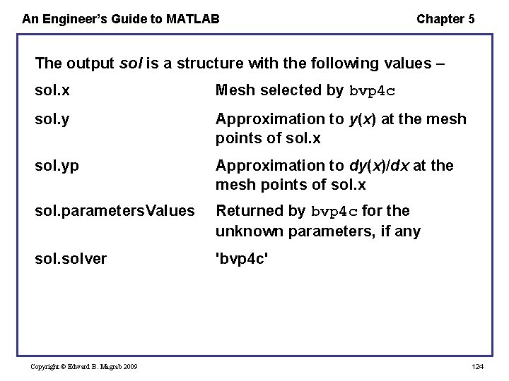
An Engineer’s Guide to MATLAB Chapter 5 The output sol is a structure with the following values – sol. x Mesh selected by bvp 4 c sol. y Approximation to y(x) at the mesh points of sol. x sol. yp Approximation to dy(x)/dx at the mesh points of sol. x sol. parameters. Values Returned by bvp 4 c for the unknown parameters, if any solver 'bvp 4 c' Copyright © Edward B. Magrab 2009 124

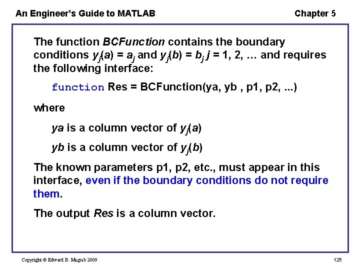
An Engineer’s Guide to MATLAB Chapter 5 The function BCFunction contains the boundary conditions yj(a) = aj and yj(b) = bj j = 1, 2, … and requires the following interface: function Res = BCFunction(ya, yb , p 1, p 2, . . . ) where ya is a column vector of yj(a) yb is a column vector of yj(b) The known parameters p 1, p 2, etc. , must appear in this interface, even if the boundary conditions do not require them. The output Res is a column vector. Copyright © Edward B. Magrab 2009 125

An Engineer’s Guide to MATLAB Chapter 5 The variable solinit is a structure obtained from the function bvpinit as solinit = bvpinit(x, y) where The vector x is a guess for the initial mesh points. The vector y is a guess of the magnitude of each of the yj. The lengths of x and y are independent of each other. The structure solinit is – x Ordered nodes of the initial mesh y Initial guess for the solution with solinit. y(: , i) a guess for the solution at the node solinit. x(i) Copyright © Edward B. Magrab 2009 126

An Engineer’s Guide to MATLAB Chapter 5 The output of bvp 4 c, sol, is a structure that contains the solution at a specific number of points. In order to obtain a smooth curve, values at additional intermediate points are needed. To provide these additional points, we use sxint = deval(sol, xint) where xint is a vector of points at which the solution is to be evaluated. sol is the output (structure) of bcp 4 c. Copyright © Edward B. Magrab 2009 127

An Engineer’s Guide to MATLAB Chapter 5 The output sxint is an array containing the values of yj at the spatial locations xint; that is, y 1(xint) = sxint(1, : ) y 2(xint) = sxint (2, : ) sxint = deval(sol, xint) … yn(xint) = sxint (n, : ) Copyright © Edward B. Magrab 2009 128

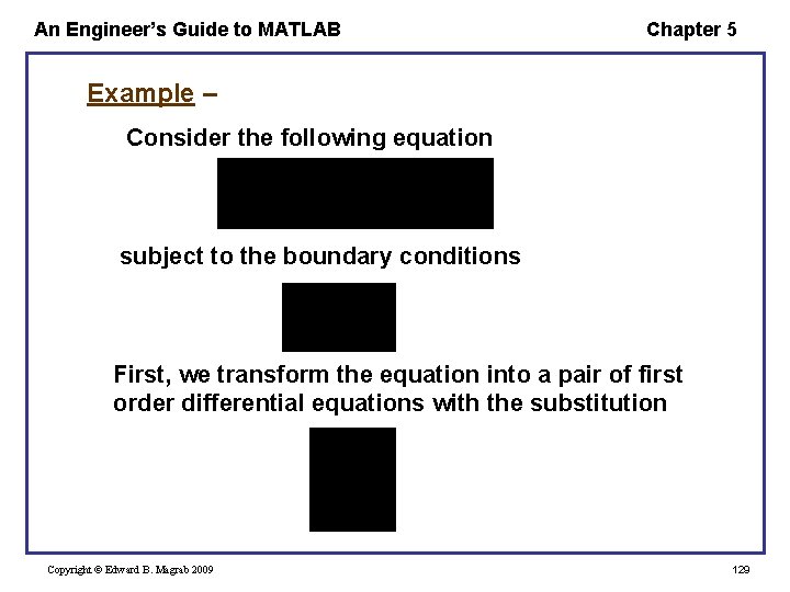
An Engineer’s Guide to MATLAB Chapter 5 Example – Consider the following equation subject to the boundary conditions First, we transform the equation into a pair of first order differential equations with the substitution Copyright © Edward B. Magrab 2009 129

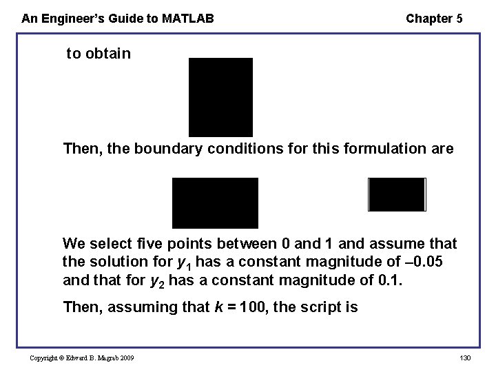
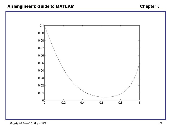
An Engineer’s Guide to MATLAB Chapter 5 to obtain Then, the boundary conditions for this formulation are We select five points between 0 and 1 and assume that the solution for y 1 has a constant magnitude of 0. 05 and that for y 2 has a constant magnitude of 0. 1. Then, assuming that k = 100, the script is Copyright © Edward B. Magrab 2009 130

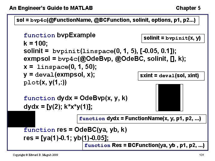
An Engineer’s Guide to MATLAB Chapter 5 sol = bvp 4 c(@Function. Name, @BCFunction, solinit, options, p 1, p 2. . . ) function bvp. Example solinit = bvpinit(x, y) k = 100; solinit = bvpinit(linspace(0, 1, 5), [-0. 05, 0. 1]); exmpsol = bvp 4 c(@Ode. Bvp, @Ode. BC, solinit, [], k); x = linspace(0, 1, 50); y = deval(exmpsol, x); sxint = deval(sol, xint) plot(x, y(1, : )) function dydx = Ode. Bvp(x, y, k) dydx = [y(2); k*x*y(1)]; function dydx = Function. Name(x, y, p 1, p 2, . . . ) function res = Ode. BC(ya, yb, k) res = [ya(1)-0. 1; yb(1)-0. 05]; function Res = BCFunction(ya, yb , p 1, p 2, . . . ) Copyright © Edward B. Magrab 2009 131

An Engineer’s Guide to MATLAB Copyright © Edward B. Magrab 2009 Chapter 5 132

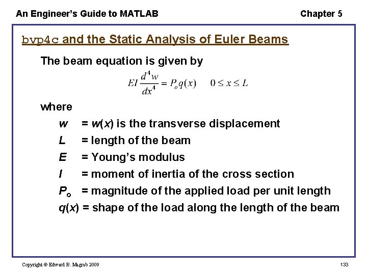
An Engineer’s Guide to MATLAB Chapter 5 bvp 4 c and the Static Analysis of Euler Beams The beam equation is given by where w = w(x) is the transverse displacement L = length of the beam E = Young’s modulus I = moment of inertia of the cross section Po = magnitude of the applied load per unit length q(x) = shape of the load along the length of the beam Copyright © Edward B. Magrab 2009 133

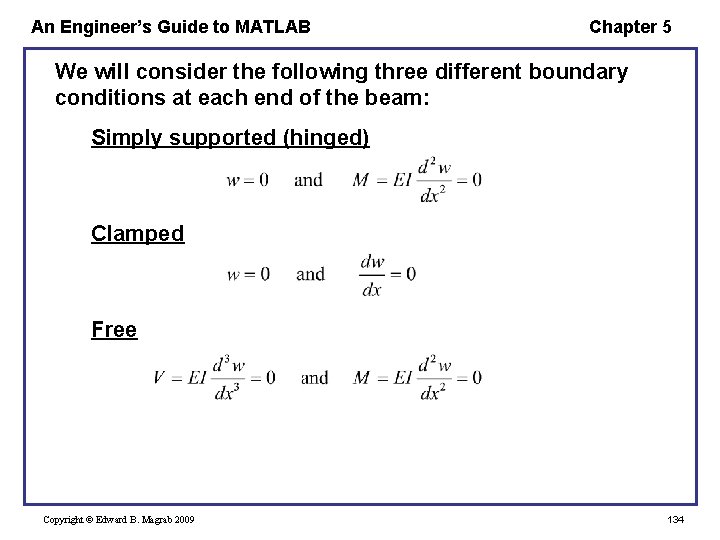
An Engineer’s Guide to MATLAB Chapter 5 We will consider the following three different boundary conditions at each end of the beam: Simply supported (hinged) Clamped Free Copyright © Edward B. Magrab 2009 134

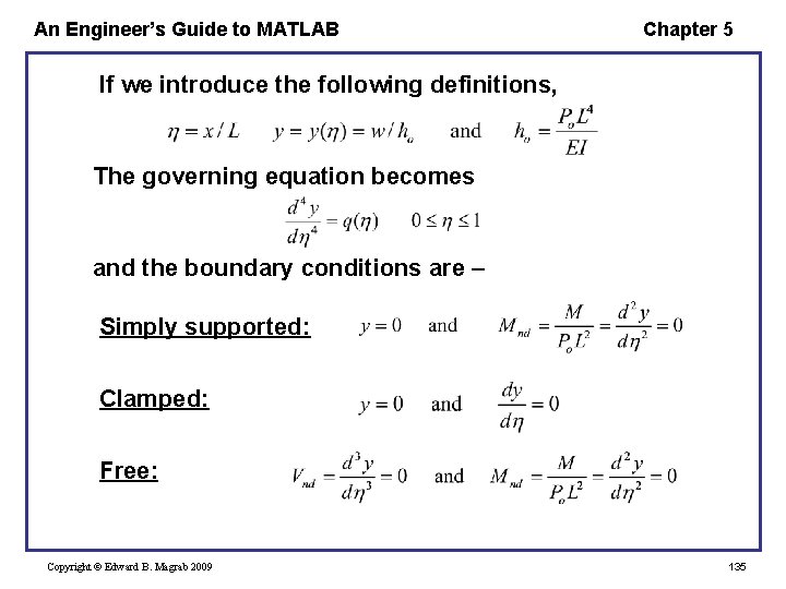
An Engineer’s Guide to MATLAB Chapter 5 If we introduce the following definitions, The governing equation becomes and the boundary conditions are – Simply supported: Clamped: Free: Copyright © Edward B. Magrab 2009 135

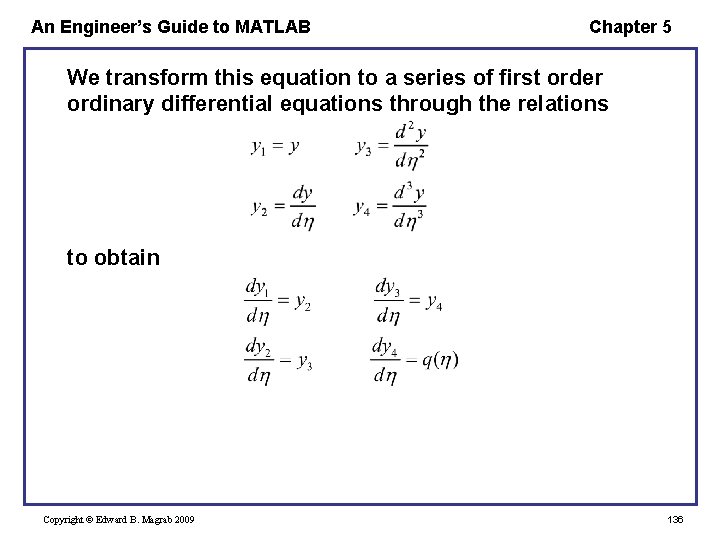
An Engineer’s Guide to MATLAB Chapter 5 We transform this equation to a series

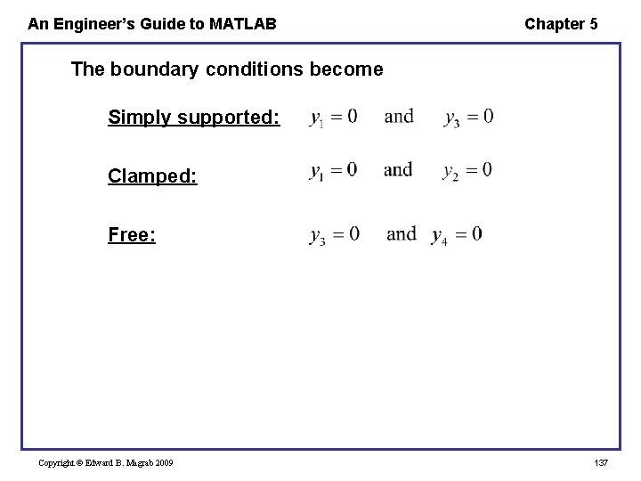
An Engineer’s Guide to MATLAB Chapter 5 The boundary conditions become Simply supported: Clamped:

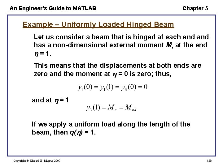
An Engineer’s Guide to MATLAB Chapter 5 Example – Uniformly Loaded Hinged Beam Let us consider a beam that is hinged at each end and has a non-dimensional external moment Mr at the end = 1. This means that the displacements at both ends are zero and the moment at = 0 is zero; thus, and at = 1 If we apply a uniform load along the length of the beam, then q( ) = 1. Copyright © Edward B. Magrab 2009 138

An Engineer’s Guide to MATLAB Chapter 5 Let us assume that Mr = 0. 8 and we have previously assumed that q = 1. We take 10 mesh points as our guess and guess that the magnitudes of the displacement, slope, moment, and shear force each have the value of 0. 5. The function that is used to represent the system of first order equations is called Beam. ODEqo and the function that represents the boundary conditions is called Beam. Hinged. BC. Then the script is Copyright © Edward B. Magrab 2009 139

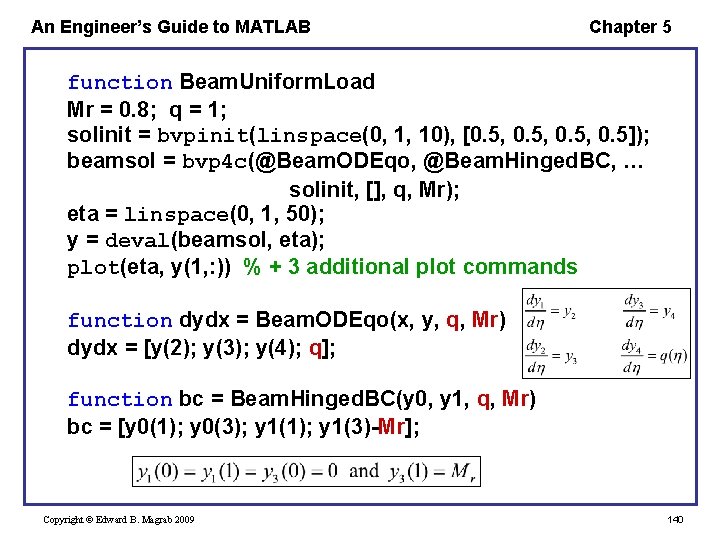
An Engineer’s Guide to MATLAB Chapter 5 function Beam. Uniform. Load Mr = 0. 8; q = 1; solinit = bvpinit(linspace(0, 1, 10), [0. 5, 0. 5]); beamsol = bvp 4 c(@Beam. ODEqo, @Beam. Hinged. BC, … solinit, [], q, Mr); eta = linspace(0, 1, 50); y = deval(beamsol, eta); plot(eta, y(1, : )) % + 3 additional plot commands function dydx = Beam. ODEqo(x, y, q, Mr) dydx = [y(2); y(3); y(4); q]; function bc = Beam. Hinged. BC(y 0, y 1, q, Mr) bc = [y 0(1); y 0(3); y 1(1); y 1(3)-Mr]; Copyright © Edward B. Magrab 2009 140

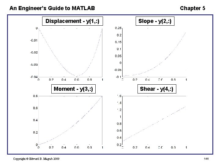
An Engineer’s Guide to MATLAB Displacement - y(1, : ) Moment - y(3, :

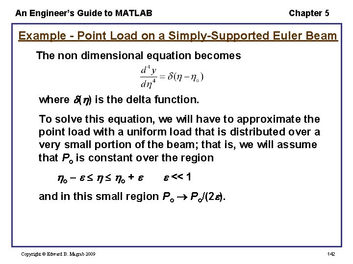
An Engineer’s Guide to MATLAB Chapter 5 Example - Point Load on a Simply-Supported Euler Beam The non dimensional equation becomes where ( ) is the delta function. To solve this equation, we will have to approximate the point load with a uniform load that is distributed over a very small portion of the beam; that is, we will assume that Po is constant over the region o o + << 1 and in this small region Po Po/(2 ). Copyright © Edward B. Magrab 2009 142

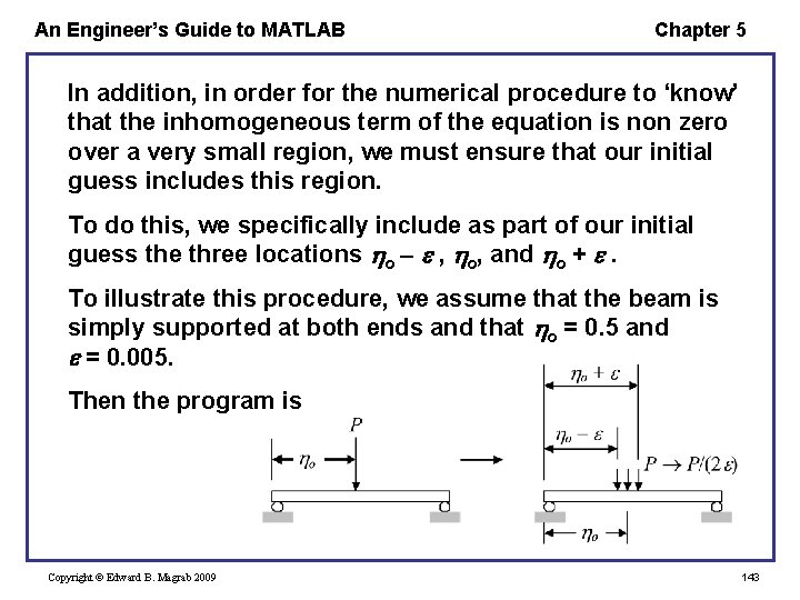
An Engineer’s Guide to MATLAB Chapter 5 In addition, in order for the numerical procedure to ‘know’ that the inhomogeneous term of the equation is non zero over a very small region, we must ensure that our initial guess includes this region. To do this, we specifically include as part of our initial guess the three locations o , o, and o + . To illustrate this procedure, we assume that the beam is simply supported at both ends and that o = 0. 5 and = 0. 005. Then the program is Copyright © Edward B. Magrab 2009 143

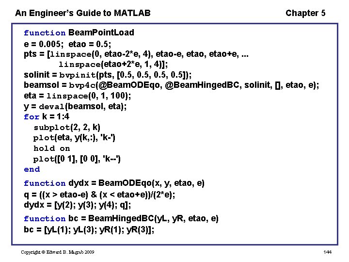
An Engineer’s Guide to MATLAB Chapter 5 function Beam. Point. Load e = 0. 005; etao = 0. 5; pts = [linspace(0, etao-2*e, 4), etao-e, etao+e, . . . linspace(etao+2*e, 1, 4)]; solinit = bvpinit(pts, [0. 5, 0. 5]); beamsol = bvp 4 c(@Beam. ODEqo, @Beam. Hinged. BC, solinit, [], etao, e); eta = linspace(0, 1, 100); y = deval(beamsol, eta); for k = 1: 4 subplot(2, 2, k) plot(eta, y(k, : ), 'k-') hold on plot([0 1], [0 0], 'k--') end function dydx = Beam. ODEqo(x, y, etao, e) q = ((x > etao-e) & (x < etao+e))/(2*e); dydx = [y(2); y(3); y(4); q]; function bc = Beam. Hinged. BC(y. L, y. R, etao, e) bc = [y. L(1); y. L(3); y. R(1); y. R(3)]; Copyright © Edward B. Magrab 2009 144

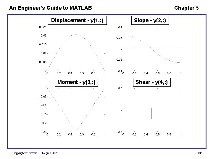
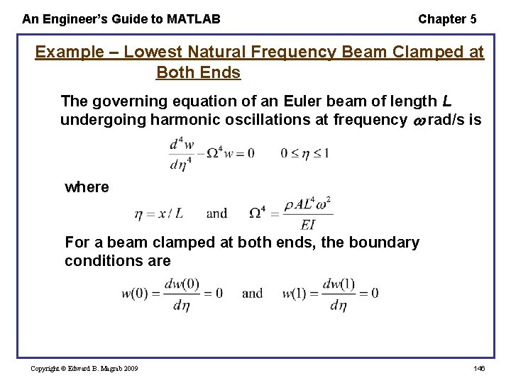
An Engineer’s Guide to MATLAB Chapter 5 Example – Lowest Natural Frequency Beam Clamped at Both Ends The governing equation of an Euler beam of length L undergoing harmonic oscillations at frequency rad/s is where For a beam clamped at both ends, the boundary conditions are Copyright © Edward B. Magrab 2009 146

An Engineer’s Guide to MATLAB Chapter 5 Making the appropriate substitutions, we obtain and Five conditions must be specified: four homogeneous boundary conditions and a fifth condition that will permit the unknown parameter to be determined. We shall choose the fifth condition as the non zero boundary condition y 4(0) = 0. 05. (The magnitude 0. 05 is not critical, but it should be ‘small’. ) Copyright © Edward B. Magrab 2009 147

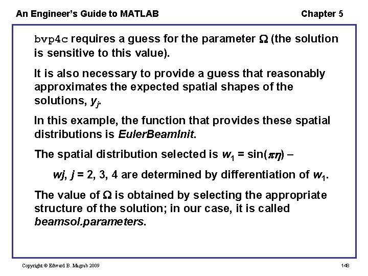
An Engineer’s Guide to MATLAB Chapter 5 bvp 4 c requires a guess for the parameter (the solution is sensitive to this value). It is also necessary to provide a guess that reasonably approximates the expected spatial shapes of the solutions, yj. In this example, the function that provides these spatial distributions is Euler. Beam. Init. The spatial distribution selected is w 1 = sin( ) – wj, j = 2, 3, 4 are determined by differentiation of w 1. The value of is obtained by selecting the appropriate structure of the solution; in our case, it is called beamsol. parameters. Copyright © Edward B. Magrab 2009 148

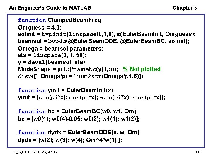
An Engineer’s Guide to MATLAB Chapter 5 function Clamped. Beam. Freq Omguess = 4. 0; solinit = bvpinit(linspace(0, 1, 6), @Euler. Beam. Init, Omguess); beamsol = bvp 4 c(@Euler. Beam. ODE, @Euler. Beam. BC, solinit); Omega = beamsol. parameters; eta = linspace(0, 1, 50); y = deval(beamsol, eta); Mode. Shape = y(1, : )/max(abs(y(1, : ))); % Not plotted disp([' Omega/pi = ' num 2 str(Omega/pi, 6)]) function yinit = Euler. Beam. Init(x) yinit = [sin(pi*x); cos(pi*x); -sin(pi*x); -cos(pi*x)]; function bc = Euler. Beam. BC(w 0, w 1, Om) bc = [w 0(1); w 0(4)-0. 05; w 0(2); w 1(1); w 1(2)]; function dydx = Euler. Beam. ODE(x, w, Om) dydx = [w(2); w(3); w(4); Om^4*w(1) ]; Copyright © Edward B. Magrab 2009 149

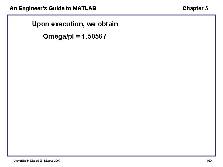
An Engineer’s Guide to MATLAB Chapter 5 Upon execution, we obtain Omega/pi = 1.

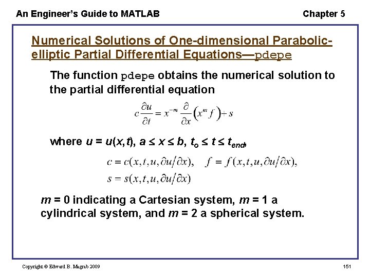
An Engineer’s Guide to MATLAB Chapter 5 Numerical Solutions of One-dimensional Parabolicelliptic Partial Differential Equations—pdepe The function pdepe obtains the numerical solution to the partial differential equation where u = u(x, t), a x b, to t tend, m = 0 indicating a Cartesian system, m = 1 a cylindrical system, and m = 2 a spherical system. Copyright © Edward B. Magrab 2009 151

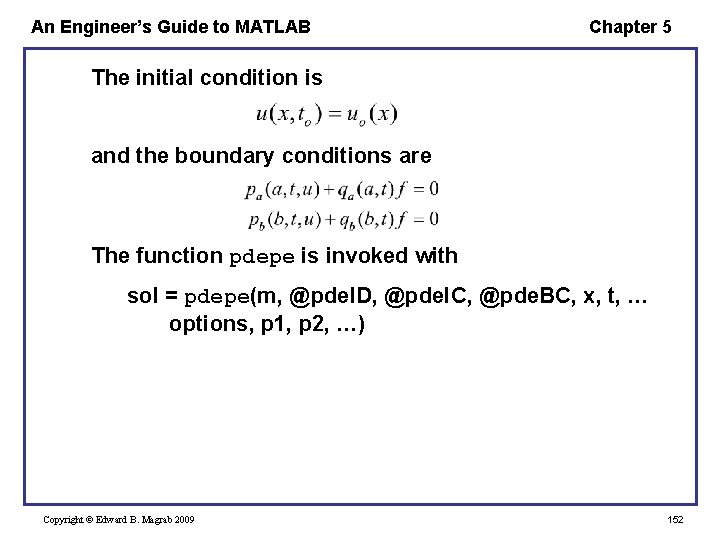
An Engineer’s Guide to MATLAB Chapter 5 The initial condition is and the boundary conditions are The function pdepe is invoked with sol = pdepe(m, @pde. ID, @pde. IC, @pde. BC, x, t, … options, p 1, p 2, …) Copyright © Edward B. Magrab 2009 152

An Engineer’s Guide to MATLAB Chapter 5 where x is a vector of values for which pdepe will provide the corresponding values of u such that x(1) = a and x(end) = b. t is a vector of values for which pdepe will provide the corresponding values of u such that t(1) = to and t(end) = tend. p 1, p 2, . . . , are parameters that are passed to pde. ID, pde. IC, and pde. BC (they must appear in each of these functions whether or not they are used by that function). options is set by odeset. Copyright © Edward B. Magrab 2009 153

An Engineer’s Guide to MATLAB Chapter 5 The quantity sol (= u(t, x)) is an array sol(i, j), where i is the element number of the temporal mesh and j is the element number of the spatial mesh. Thus, sol(i, : ) approximates u(t, x) at time ti at all mesh points from x(1) = a to x(end) = b. The function pde 1 D specifies c, f, and s as follows: function [c, f, s] = pde 1 D(x, t, u, dudx, p 1, p 2, . . . ) c= ; f= ; s= ; where dudx is the partial derivative of u with respect to x and is provided by pdepe. Copyright © Edward B. Magrab 2009 154

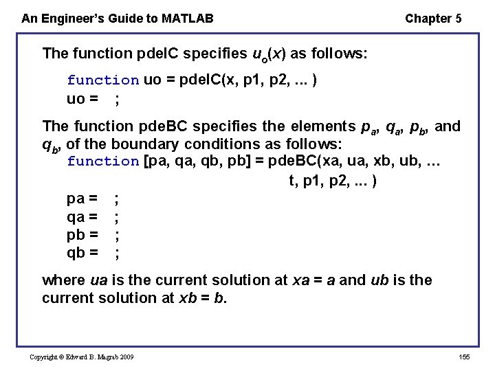
An Engineer’s Guide to MATLAB Chapter 5 The function pde. IC specifies uo(x) as follows: function uo = pde. IC(x, p 1, p 2, . . . ) uo = ; The function pde. BC specifies the elements pa, qa, pb, and qb, of the boundary conditions as follows: function [pa, qb, pb] = pde. BC(xa, ua, xb, ub, … t, p 1, p 2, . . . ) pa = ; qa = ; pb = ; qb = ; where ua is the current solution at xa = a and ub is the current solution at xb = b. Copyright © Edward B. Magrab 2009 155

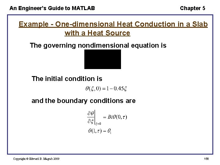
An Engineer’s Guide to MATLAB Chapter 5 Example - One-dimensional Heat Conduction in a Slab with a Heat Source The governing nondimensional equation is The initial condition is and the boundary conditions are Copyright © Edward B. Magrab 2009 156

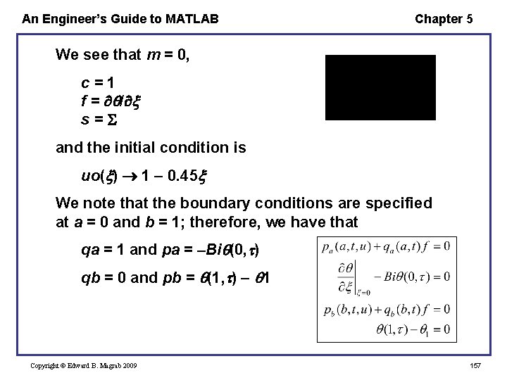
An Engineer’s Guide to MATLAB Chapter 5 We see that m = 0, c=1 f = / s= and the initial condition is uo( ) 1 0. 45 We note that the boundary conditions are specified at a = 0 and b = 1; therefore, we have that qa = 1 and pa = Bi (0, ) qb = 0 and pb = (1, ) 1 Copyright © Edward B. Magrab 2009 157

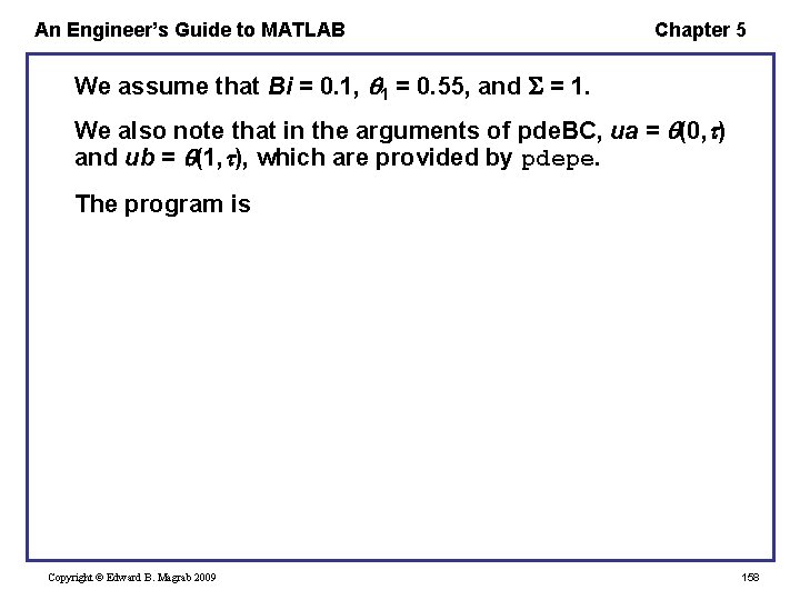
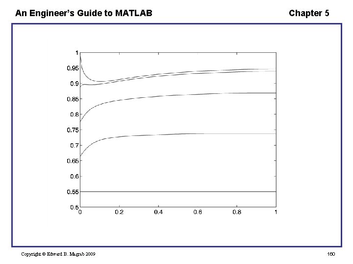
An Engineer’s Guide to MATLAB Chapter 5 We assume that Bi = 0. 1, 1 = 0. 55, and = 1. We also note that in the arguments of pde. BC, ua = (0, ) and ub = (1, ), which are provided by pdepe. The program is Copyright © Edward B. Magrab 2009 158

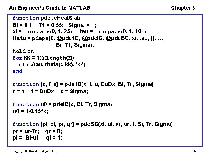
An Engineer’s Guide to MATLAB Chapter 5 function pdepe. Heat. Slab Bi = 0. 1; T 1 = 0. 55; Sigma = 1; xi = linspace(0, 1, 25); tau = linspace(0, 1, 101); theta = pdepe(0, @pde 1 D, @pde. IC, @pde. BC, xi, tau, [], … Bi, T 1, Sigma); hold on for kk = 1: 5: length(zi) plot(tau, theta(: , kk), 'k-') end function [c, f, s] = pde 1 D(x, t, u, Du. Dx, Bi, Tr, Sigma) c = 1; f = Du. Dx; s = Sigma; function u 0 = pde. IC(x, Bi, Tr, Sigma) u 0 = 1 -0. 45*x; function [pl, ql, pr, qr] = pde. BC(xl, ul, xr, ur, t, Bi, Tr, Sigma) pr = ur-Tr; qr = 0; pl = -Bi*ul; ql = 1; Copyright © Edward B. Magrab 2009 159

An Engineer’s Guide to MATLAB Copyright © Edward B. Magrab 2009 Chapter 5 160

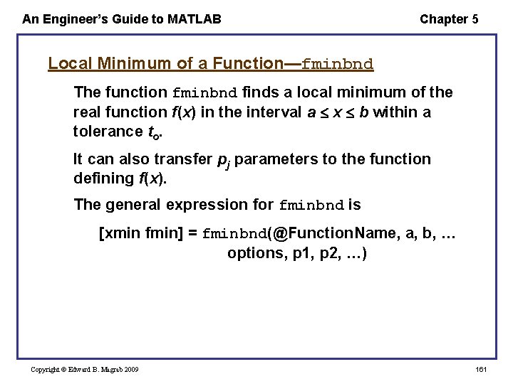
An Engineer’s Guide to MATLAB Chapter 5 Local Minimum of a Function—fminbnd The function fminbnd finds a local minimum of the real function f(x) in the interval a x b within a tolerance to. It can also transfer pj parameters to the function defining f(x). The general expression for fminbnd is [xmin fmin] = fminbnd(@Function. Name, a, b, … options, p 1, p 2, …) Copyright © Edward B. Magrab 2009 161

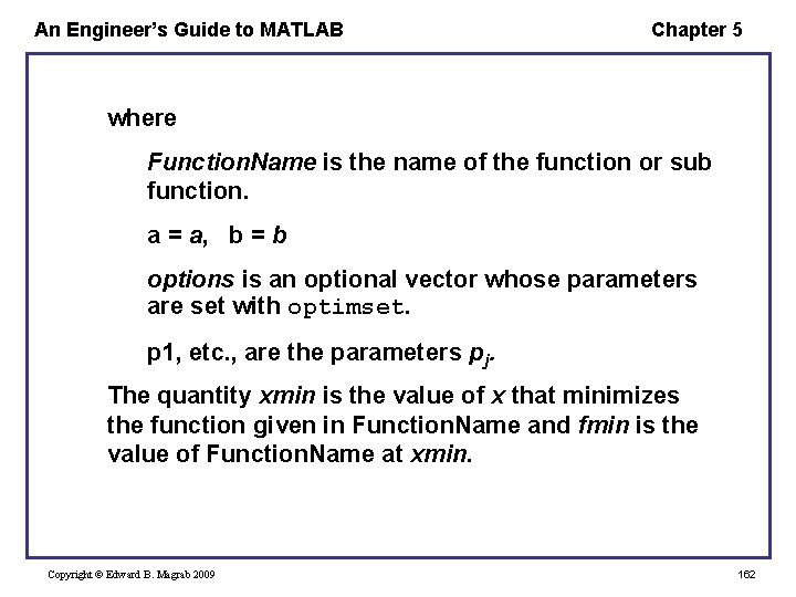
An Engineer’s Guide to MATLAB Chapter 5 where Function. Name is the name of the function or sub function. a = a, b = b options is an optional vector whose parameters are set with optimset. p 1, etc. , are the parameters pj. The quantity xmin is the value of x that minimizes the function given in Function. Name and fmin is the value of Function. Name at xmin. Copyright © Edward B. Magrab 2009 162

An Engineer’s Guide to MATLAB Chapter 5 The interface for Function. Name has the form function z = Function. Name(x, p 1, p 2, . . . ) where x is the independent variable that fminbnd is varying in order to minimize f(x). The independent variable must always appear in the first location. When f(x) is an expression that is represented by inline or an anonymous function with the name Ior. AFunction. Name, fminbnd is accessed as [xmin, fmin] = fminbnd(Ior. AFunction. Name, a, b, … options, p 1, p 2, …) Copyright © Edward B. Magrab 2009 163

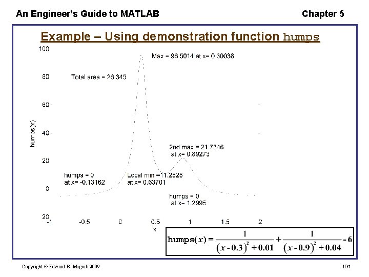
An Engineer’s Guide to MATLAB Chapter 5 Example – Using demonstration function humps Copyright

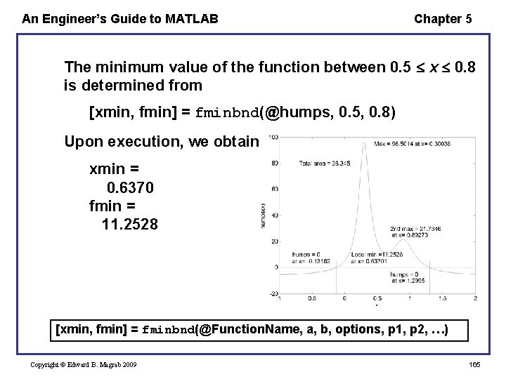
An Engineer’s Guide to MATLAB Chapter 5 The minimum value of the function between 0. 5 x 0. 8 is determined from [xmin, fmin] = fminbnd(@humps, 0. 5, 0. 8) Upon execution, we obtain xmin = 0. 6370 fmin = 11. 2528 [xmin, fmin] = fminbnd(@Function. Name, a, b, options, p 1, p 2, …) Copyright © Edward B. Magrab 2009 165

An Engineer’s Guide to MATLAB Chapter 5 To determine the maximum value of humps in the interval 0 x 0. 5 and where it occurs, we have to recognize that fminbnd must operate on the negative or the reciprocal of the function humps. Thus, we use inline to create a function that computes the negative of humps in this region. The script is Copyright © Edward B. Magrab 2009 166

An Engineer’s Guide to MATLAB Chapter 5 [xmax, fmax] = fminbnd(inline('-humps(x)', 'x '), 0, 0. 5); disp(['Maximum value of humps in the interval 0 <= x <= 0. 5 is ' num 2 str(-fmax)]) disp(['which occurs at x = ' num 2 str(xmax)]) which, upon execution, displays Maximum value of humps in the interval 0 <= x <= 0. 5 is 96. 50 which occurs at x = 0. 30039 [xmin, fmin] = fminbnd(Ior. AFunction. Name, a, b, options, p 1, p 2, …) Copyright © Edward B. Magrab 2009 167

An Engineer’s Guide to MATLAB Chapter 5 Symbolic Solutions and Converting Symbolic Expressions into Functions One way to convert a symbolic expression f into a function, we employ inline and vectorize(f) which converts its argument to a string and converts the multiplication, division, and exponentiation operators to their dot operator counterparts. Copyright © Edward B. Magrab 2009 168

An Engineer’s Guide to MATLAB Chapter 5 A second way is to use matlab. Function to create an anonymous function. If f = f(x, y, z) is a symbolic expression with symbolic variables x, y, and z, then fnct = matlab. Function(f, 'vars', [x, y, z]) where 'vars' (apostrophes required) indicates that an anonymous function will be created with the parameters x, y, z of the form fnct = @(x, y, z) (f) where f is a Matlab expression with the *, /, and ^ operators replaced by their dot operation counterpart; that is, by. *, . /, and. ^. Copyright © Edward B. Magrab 2009 169

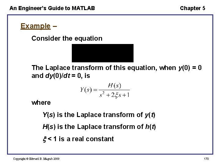
An Engineer’s Guide to MATLAB Chapter 5 Example – Consider the equation The Laplace transform of this equation, when y(0) = 0 and dy(0)/dt = 0, is where Y(s) is the Laplace transform of y(t) H(s) is the Laplace transform of h(t) < 1 is a real constant Copyright © Edward B. Magrab 2009 170

An Engineer’s Guide to MATLAB Chapter 5 If we assume that h(t) = u(t) where u(t) is the unit step function, then H(s) = 1/s The script to determine y(t) is syms xi t real den = s*(s^2+2*xi*s+1); yt = ilaplace(1/den, s, t); yt=simple(yt) where simple put yt in its simplest form. Copyright © Edward B. Magrab 2009 171

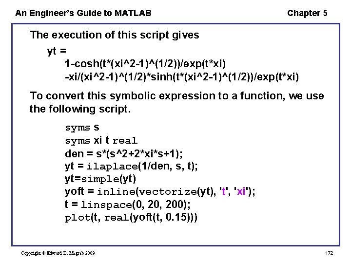
An Engineer’s Guide to MATLAB Chapter 5 The execution of this script gives yt = 1 -cosh(t*(xi^2 -1)^(1/2))/exp(t*xi) -xi/(xi^2 -1)^(1/2)*sinh(t*(xi^2 -1)^(1/2))/exp(t*xi) To convert this symbolic expression to a function, we use the following script. syms s syms xi t real den = s*(s^2+2*xi*s+1); yt = ilaplace(1/den, s, t); yt=simple(yt) yoft = inline(vectorize(yt), 't', 'xi'); t = linspace(0, 200); plot(t, real(yoft(t, 0. 15))) Copyright © Edward B. Magrab 2009 172

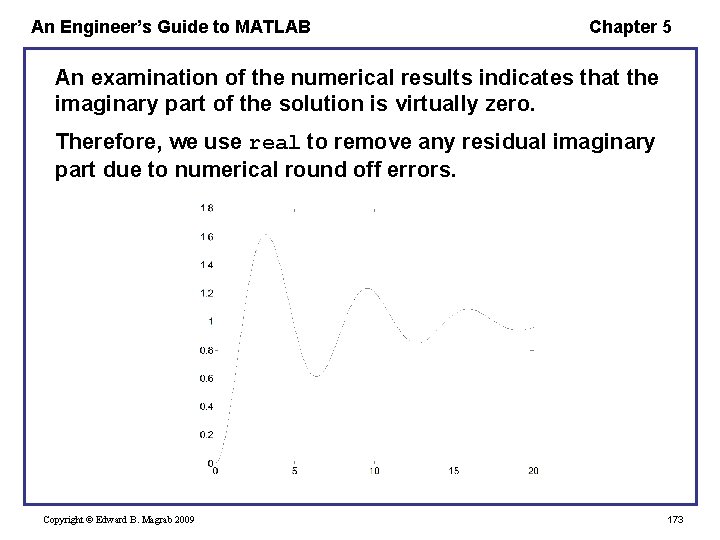
An Engineer’s Guide to MATLAB Chapter 5 An examination of the numerical results indicates that the imaginary part of the solution is virtually zero. Therefore, we use real to remove any residual imaginary part due to numerical round off errors. Copyright © Edward B. Magrab 2009 173

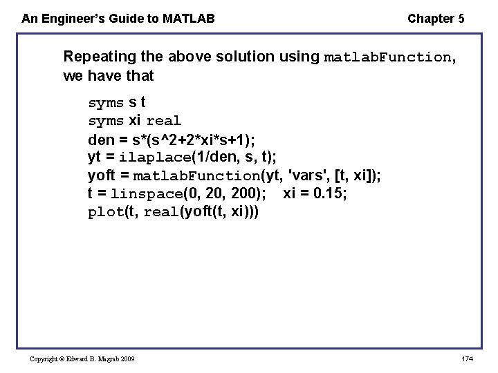
An Engineer’s Guide to MATLAB Chapter 5 Repeating the above solution using matlab. Function, we have that syms s t syms xi real den = s*(s^2+2*xi*s+1); yt = ilaplace(1/den, s, t); yoft = matlab. Function(yt, 'vars', [t, xi]); t = linspace(0, 200); xi = 0. 15; plot(t, real(yoft(t, xi))) Copyright © Edward B. Magrab 2009 174