An app thought An app thought VC question

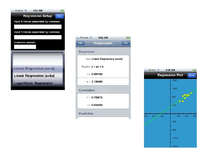
An “app” thought!

An “app” thought! VC question: How much is this worth as a killer app?

GAUSS, Carl Friedrich 1777 -1855 http: //www. york. ac. uk/depts/maths/histstat/people/

1 f(X) = e-(X - ) / 22 2 Where = 3. 1416 and e = 2. 7183 2

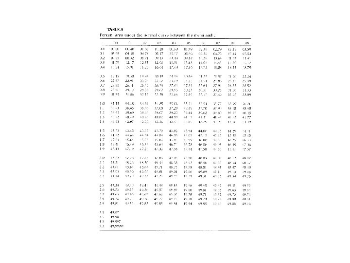
Normal Distribution Unimodal Symmetrical 34. 13% of area under curve is between µ and +1 34. 13% of area under curve is between µ and -1 68. 26% of area under curve is within 1 of µ. 95. 44% of area under curve is within 2 of µ.

Some Problems • If z = 1, what % of the normal curve lies above it? Below it? • If z = -1. 7, what % of the normal curve lies below it? • What % of the curve lies between z = -. 75 and z =. 75? • What is the z-score such that only 5% of the curve lies above it? • In the SAT with µ=500 and =100, what % of the population do you expect to score above 600? Above 750?

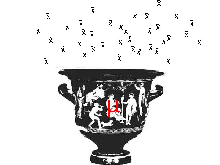
Sample _ C XC Sample _ D XD s d n sc n Population µ Sample _ B n Sample _ E XE se n Sample _ A XA s a n In reality, the sample mean is just one of many possible sample means drawn from the population, and is rarely equal to µ. XB s b

_ C Sample XC _ D Sample XD s d n sc n Population µ _ B Sample n _ E Sample XE se n _ A Sample XA s a n In reality, the sample sd is also just one of many possible sample sd’s drawn from the population, and is rarely equal to σ. XB s b

What’s the difference? s 2 SS = (N - 1) 2 SS = N

What’s the difference? (occasionally you will see this little “hat” on the symbol to clearly indicate that this is a variance estimate) – I like this because it is a reminder that we are usually just making estimates, and estimates are always accompanied by error and bias, and that’s one of the enduring lessons of statistics) ^2 s SS = (N - 1) 2 SS = N

Standard deviation. s = SS (N - 1)

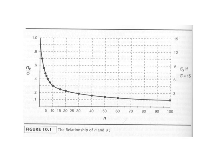
As sample size increases, the magnitude of the sampling error decreases; at a certain point, there are diminishing returns of increasing sample size to decrease sampling error.

Central Limit Theorem The sampling distribution of means from random samples of n observations approaches a normal distribution regardless of the shape of the parent population. Just for fun, go check out the Khan Academy http: //www. khanacademy. org/video/central-limit-theorem? playlist=Statistics

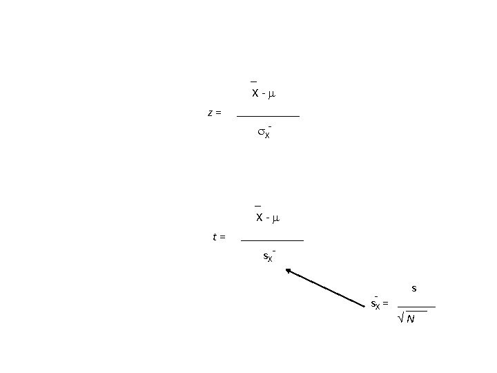
Wow! We can use the z-distribution to test a hypothesis. _ X- z= X-

Step 1. State the statistical hypothesis H 0 to be tested (e. g. , H 0: = 100) Step 2. Specify the degree of risk of a type-I error, that is, the risk of incorrectly concluding that H 0 is false when it is true. This risk, stated as a probability, is denoted by , the probability of a Type I error. Step 3. Assuming H 0 to be correct, find the probability of obtaining a sample mean that differs from by an amount as large or larger than what was observed. Step 4. Make a decision regarding H 0, whether to reject or not to reject it.

An Example You draw a sample of 25 adopted children. You are interested in whether they are different from the general population on an IQ test ( = 100, = 15). The mean from your sample is 108. What is the null hypothesis?

An Example You draw a sample of 25 adopted children. You are interested in whether they are different from the general population on an IQ test ( = 100, = 15). The mean from your sample is 108. What is the null hypothesis? H 0: = 100

An Example You draw a sample of 25 adopted children. You are interested in whether they are different from the general population on an IQ test ( = 100, = 15). The mean from your sample is 108. What is the null hypothesis? H 0: = 100 Test this hypothesis at =. 05

An Example You draw a sample of 25 adopted children. You are interested in whether they are different from the general population on an IQ test ( = 100, = 15). The mean from your sample is 108. What is the null hypothesis? H 0: = 100 Test this hypothesis at =. 05 Step 3. Assuming H 0 to be correct, find the probability of obtaining a sample mean that differs from by an amount as large or larger than what was observed. Step 4. Make a decision regarding H 0, whether to reject or not to reject it.

GOSSET, William Sealy 1876 -1937

GOSSET, William Sealy 1876 -1937

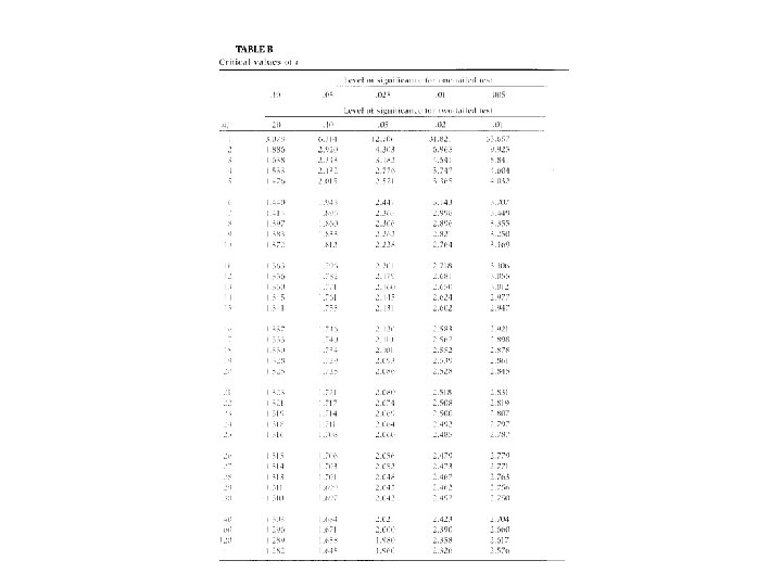
The t-distribution is a family of distributions varying by degrees of freedom (d. f. , where d. f. =n-1). At d. f. = , but at smaller than that, the tails are fatter.

The t-distribution is a family of distributions varying by degrees of freedom (d. f. , where d. f. =n-1). At d. f. = , but at smaller than that, the tails are fatter.

Degrees of Freedom df = N - 1

Problem Sample: Mean = 54. 2 SD = 2. 4 N = 16 Do you think that this sample could have been drawn from a population with = 50?

Problem Sample: Mean = 54. 2 SD = 2. 4 N = 16 Do you think that this sample could have been drawn from a population with = 50? _ X- t= s. X-

The mean for the sample of 54. 2 (sd = 2. 4) was significantly different from a hypothesized population mean of 50, t(15) = 7. 0, p <. 001.

The mean for the sample of 54. 2 (sd = 2. 4) was significantly reliably different from a hypothesized population mean of 50, t(15) = 7. 0, p <. 001.

Sample. C r. XY Sample. D Population r. XY _ Sample. E r. XY Sample. B r. XY Sample. A r. XY

The t distribution, at N-2 degrees of freedom, can be used to test the probability that the statistic r was drawn from a population with = 0. Table C. H 0 : XY = 0 H 1 : XY 0 where r N-2 t= 1 - r 2