An ALPS view of Sparse Recovery Volkan Cevher

An ALPS’ view of Sparse Recovery Volkan Cevher volkan. cevher@epfl. ch Laboratory for Information and Inference Systems - LIONS http: //lions. epfl. ch

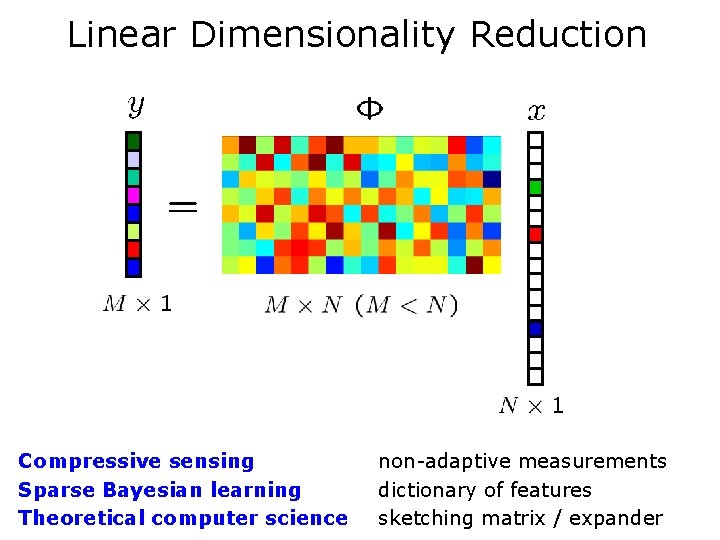
Linear Dimensionality Reduction Compressive sensing Sparse Bayesian learning Theoretical computer science non-adaptive measurements dictionary of features sketching matrix / expander

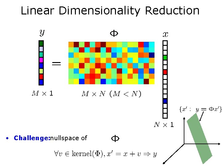
Linear Dimensionality Reduction • Challenge: nullspace of

A Deterministic View Compressive Sensing

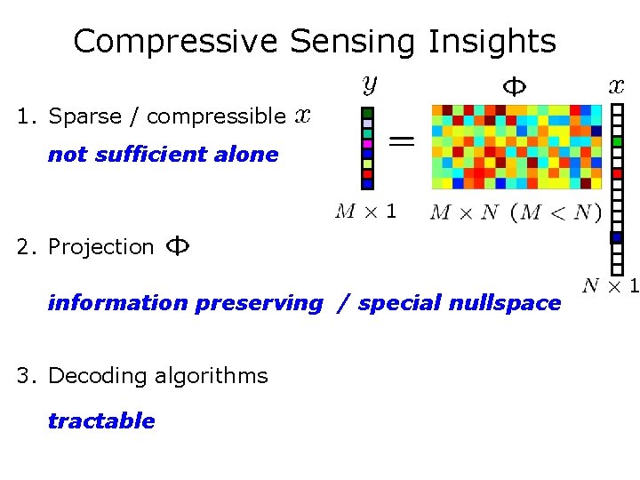
Compressive Sensing Insights 1. Sparse / compressible not sufficient alone 2. Projection information preserving / special nullspace 3. Decoding algorithms tractable

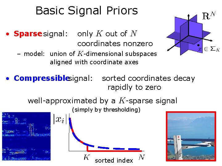
Basic Signal Priors • Sparse signal: only K out of N coordinates nonzero – model: union of K-dimensional subspaces aligned with coordinate axes • Compressiblesignal: sorted coordinates decay rapidly to zero well-approximated by a K-sparse signal (simply by thresholding) sorted index

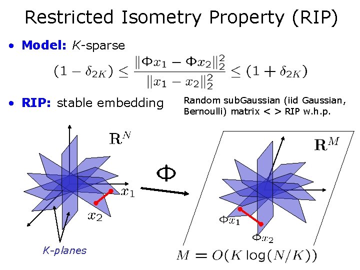
Restricted Isometry Property (RIP) • Model: K-sparse • RIP: stable embedding K-planes Random sub. Gaussian (iid Gaussian, Bernoulli) matrix < > RIP w. h. p.

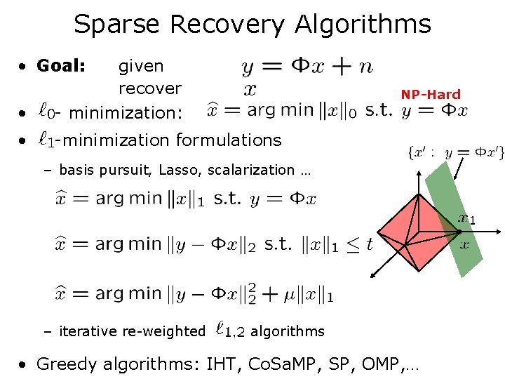
Sparse Recovery Algorithms • Goal: • given recover - minimization: • -minimization formulations NP-Hard – basis pursuit, Lasso, scalarization … – iterative re-weighted algorithms • Greedy algorithms: IHT, Co. Sa. MP, SP, OMP, …

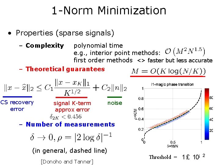
1 -Norm Minimization • Properties (sparse signals) – Complexity polynomial time e. g. , interior point methods: first order methods <> faster but less accurate – Theoretical guarantees CS recovery error signal K-term approx error noise – Number of measurements (in general, dashed line) [Donoho and Tanner] Threshold =

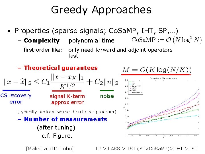
Greedy Approaches • Properties (sparse signals; Co. Sa. MP, IHT, SP, …) – Complexity first-order like: polynomial time only need forward and adjoint operators fast – Theoretical guarantees CS recovery error signal K-term approx error noise (typically perform worse than linear program) – Number of measurements (after tuning) c. f. Figure. [Maleki and Donoho] LP > LARS > TST (SP>Co. Sa. MP)> IHT > IST

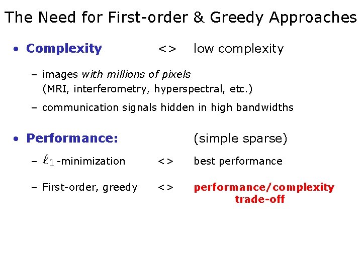
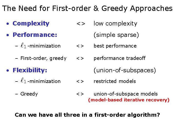
The Need for First-order & Greedy Approaches • Complexity <> low complexity – images with millions of pixels (MRI, interferometry, hyperspectral, etc. ) – communication signals hidden in high bandwidths • Performance: – -minimization – First-order, greedy (simple sparse) <> best performance <> performance/complexity trade-off

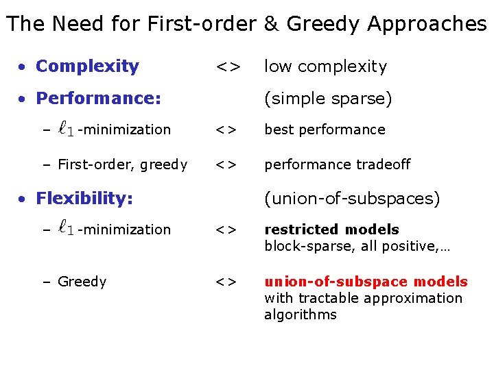
The Need for First-order & Greedy Approaches • Complexity <> • Performance: – -minimization – First-order, greedy (simple sparse) <> best performance <> performance tradeoff • Flexibility: – -minimization – Greedy low complexity (union-of-subspaces) <> restricted models block-sparse, all positive, … <> union-of-subspace models with tractable approximation algorithms

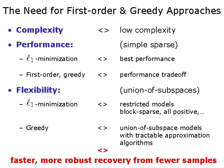
The Need for First-order & Greedy Approaches • Complexity <> • Performance: – -minimization – First-order, greedy (simple sparse) <> best performance <> performance tradeoff • Flexibility: – -minimization – Greedy low complexity (union-of-subspaces) <> restricted models block-sparse, all positive, … <> union-of-subspace models with tractable approximation algorithms <> faster, more robust recovery from fewer samples

The Need for First-order & Greedy Approaches • Complexity <> • Performance: – -minimization – First-order, greedy (simple sparse) <> best performance <> performance tradeoff • Flexibility: – -minimization – Greedy low complexity (union-of-subspaces) <> restricted models <> union-of-subspace models (model-based iterative recovery) Can we have all three in a first-order algorithm?

ENTER Algebraic Pursuits— ALPS

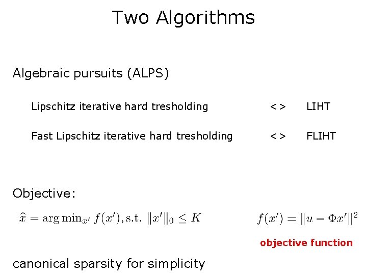
Two Algorithms Algebraic pursuits (ALPS) Lipschitz iterative hard tresholding <> LIHT Fast Lipschitz iterative hard tresholding <> FLIHT Objective: objective function canonical sparsity for simplicity

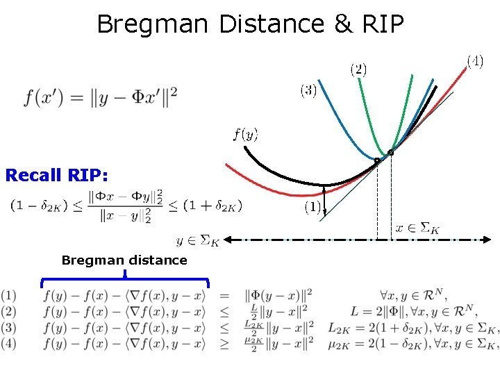
Bregman Distance & RIP Recall RIP: Bregman distance

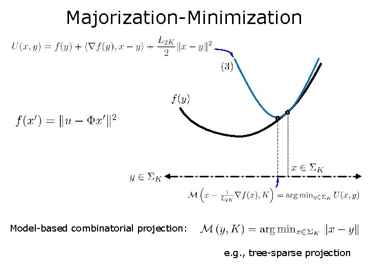
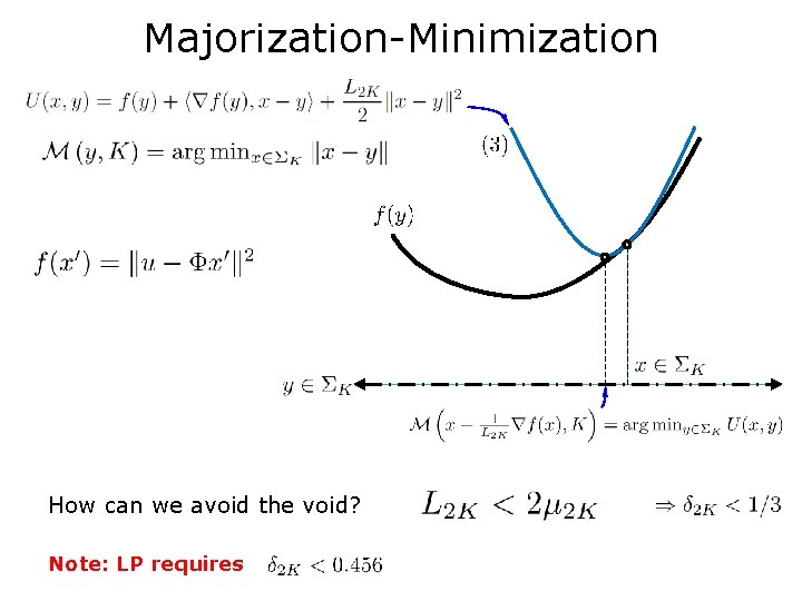
Majorization-Minimization Model-based combinatorial projection: e. g. , tree-sparse projection

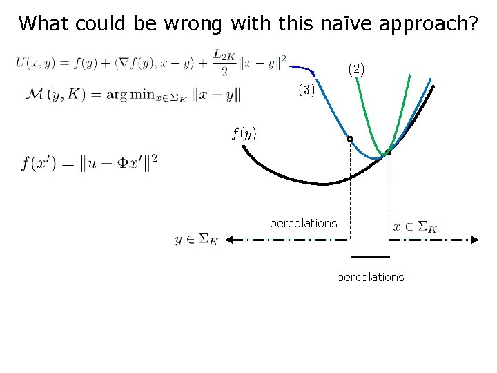
What could be wrong with this naïve approach? percolations

Majorization-Minimization How can we avoid the void? Note: LP requires

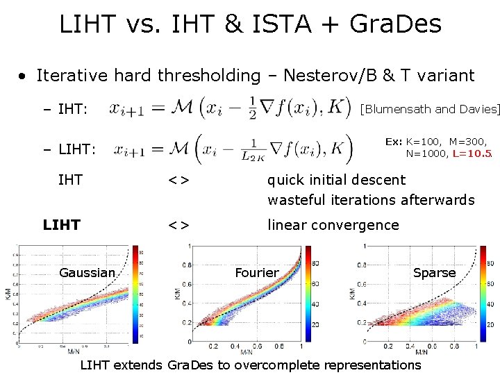
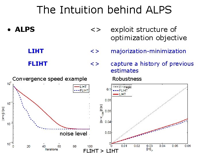
LIHT vs. IHT & ISTA + Gra. Des • Iterative hard thresholding – Nesterov/B & T variant – IHT: [Blumensath and Davies] Ex: K=100, M=300, N=1000, L=10. 5. – LIHT: IHT <> quick initial descent wasteful iterations afterwards LIHT <> linear convergence Gaussian Fourier Sparse LIHT extends Gra. Des to overcomplete representations

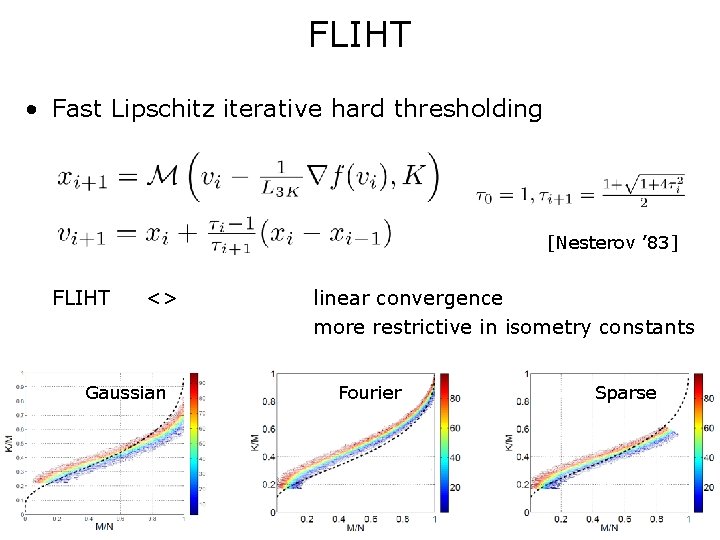
FLIHT • Fast Lipschitz iterative hard thresholding [Nesterov ’ 83] FLIHT <> Gaussian linear convergence more restrictive in isometry constants Fourier Sparse

The Intuition behind ALPS • ALPS <> exploit structure of optimization objective LIHT <> majorization-minimization FLIHT <> capture a history of previous estimates Convergence speed example Robustness noise level FLIHT > LIHT

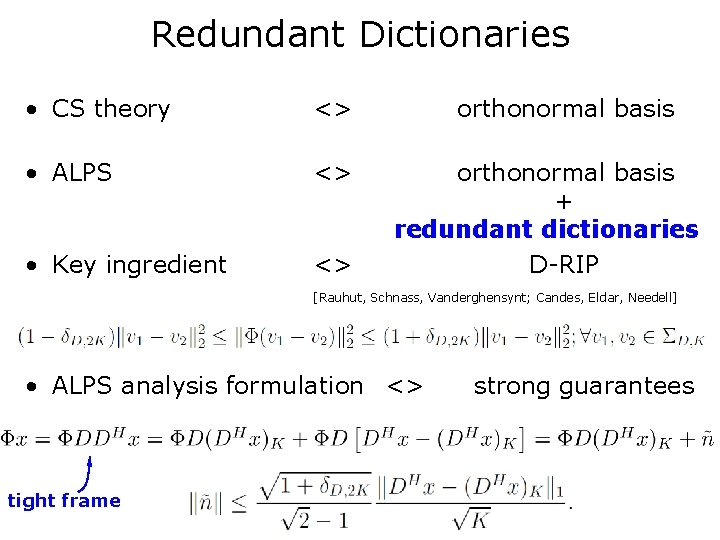
Redundant Dictionaries • CS theory <> • ALPS <> • Key ingredient <> orthonormal basis + redundant dictionaries D-RIP [Rauhut, Schnass, Vanderghensynt; Candes, Eldar, Needell] • ALPS analysis formulation <> tight frame strong guarantees

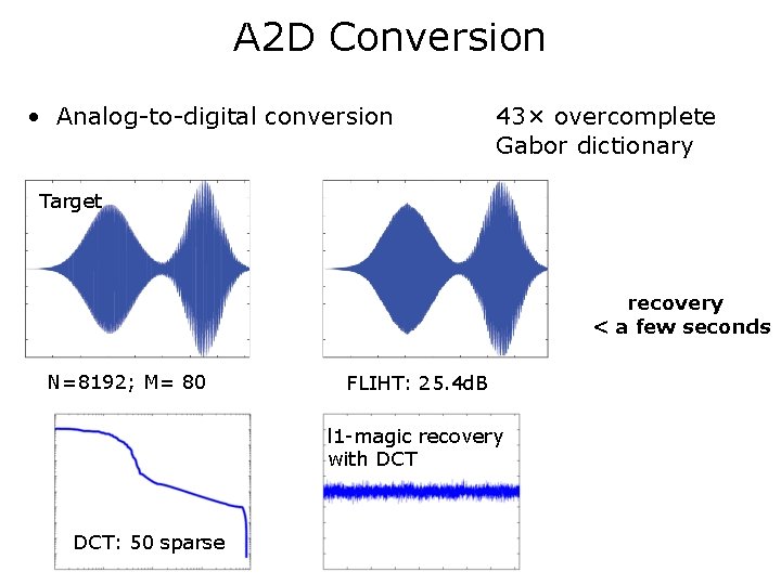
A 2 D Conversion • Analog-to-digital conversion 43× overcomplete Gabor dictionary Target recovery < a few seconds N=8192; M= 80 FLIHT: 25. 4 d. B l 1 -magic recovery with DCT: 50 sparse

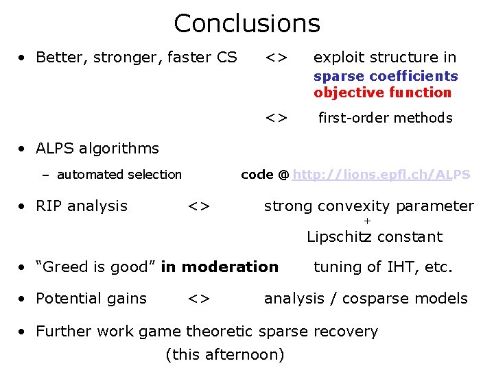
Conclusions • Better, stronger, faster CS <> exploit structure in sparse coefficients objective function <> first-order methods • ALPS algorithms – automated selection • RIP analysis code @ http: //lions. epfl. ch/ALPS <> strong convexity parameter + Lipschitz constant • “Greed is good” in moderation • Potential gains <> tuning of IHT, etc. analysis / cosparse models • Further work game theoretic sparse recovery (this afternoon)