An Adaptive Multigrid Solver for Applications in Computer

An Adaptive Multigrid Solver for Applications in Computer Graphics Misha Kazhdan and Hugues Hoppe

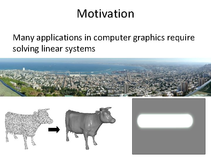
Motivation Many applications in computer graphics require solving linear systems at high resolution

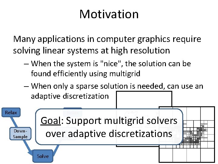
Motivation Many applications in computer graphics require solving linear systems at high resolution – When the system is "nice", the solution can be found efficiently using multigrid – When only a sparse solution is needed, can use an adaptive discretization Relax Down. Sample Relax Goal: Support multigrid solvers Upover adaptive discretizations Sample Solve

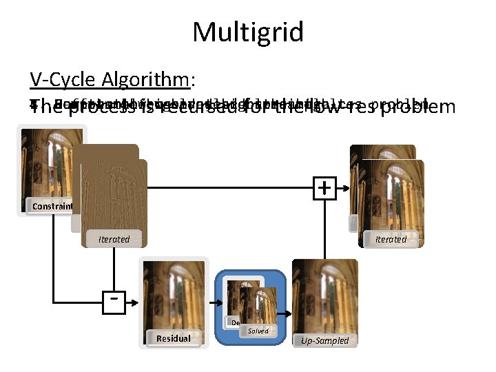
Multigrid V-Cycle Algorithm: 3. 2. 5. 1. 4. Down-sample, Compute Refine Perform Sum thethe a few low-res high-res residual solve, updates and problem high-res constraints onup-sample the results high-res problem The process is recursed for the low-res problem + Constraint Best-Guess Iterated Residual Desired Solved Up-Sampled

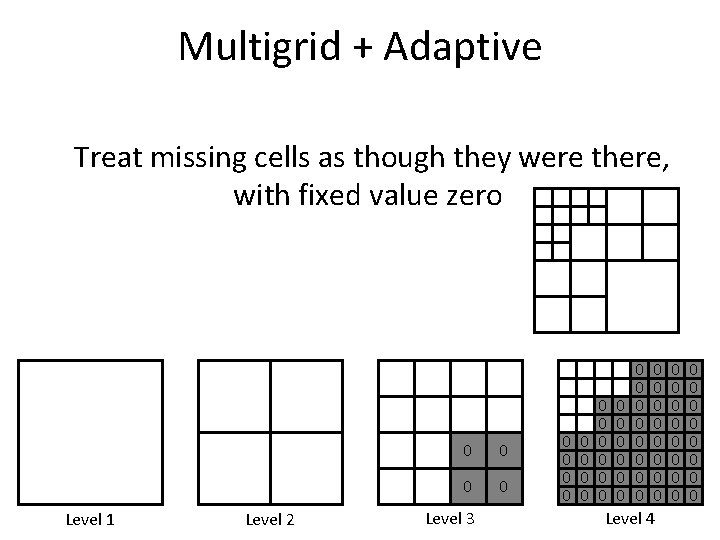
Multigrid + Adaptive Treat missing cells as though they were there, with fixed value zero Level 1 Level 2 0 0 Level 3 0 0 0 0 0 0 0 0 0 Level 4 0 0 0 0

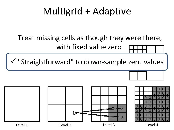
Multigrid + Adaptive Treat missing cells as though they were there, with fixed value zero "Straightforward" to down-sample zero values Level 1 Level 2 0 0 0 Level 3 0 0 0 0 0 0 0 0 0 Level 4 0 0 0 0

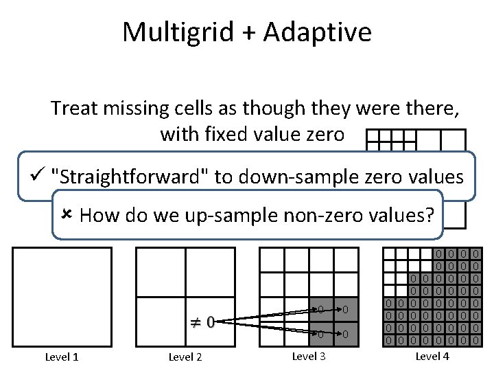
Multigrid + Adaptive Treat missing cells as though they were there, with fixed value zero "Straightforward" to down-sample zero values How do we up-sample non-zero values? Level 1 Level 2 0 0 0 Level 3 0 0 0 0 0 0 0 0 0 Level 4 0 0 0 0

Outline • • • Motivation Multigrid revisited Challenges Applications Conclusion

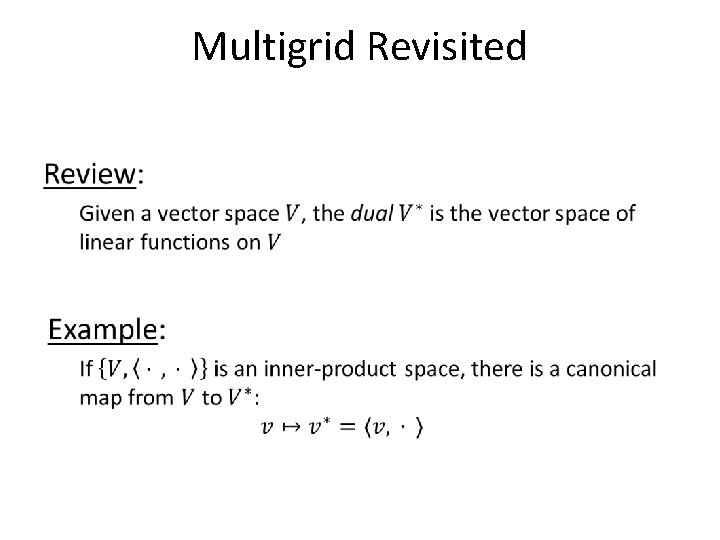
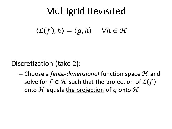
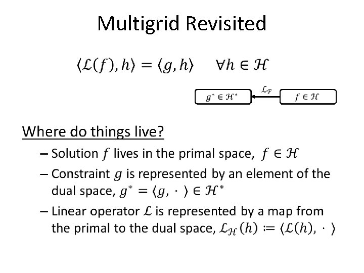
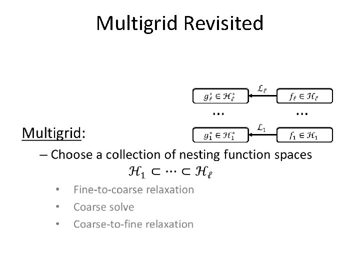
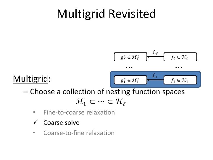
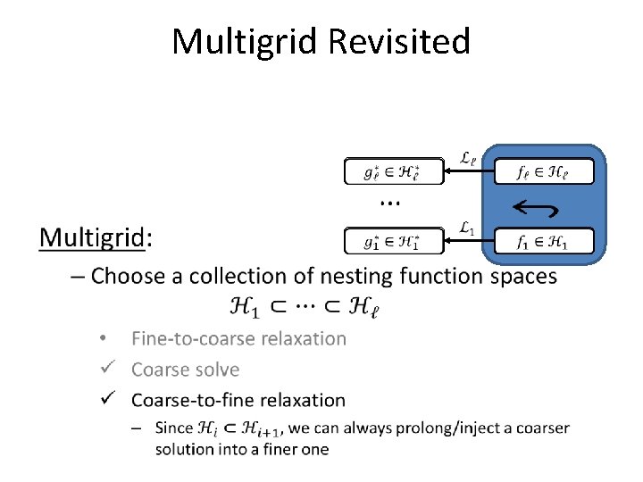
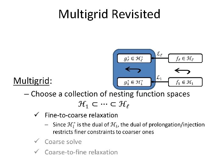
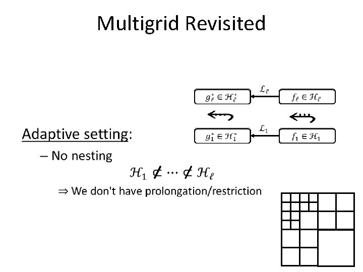
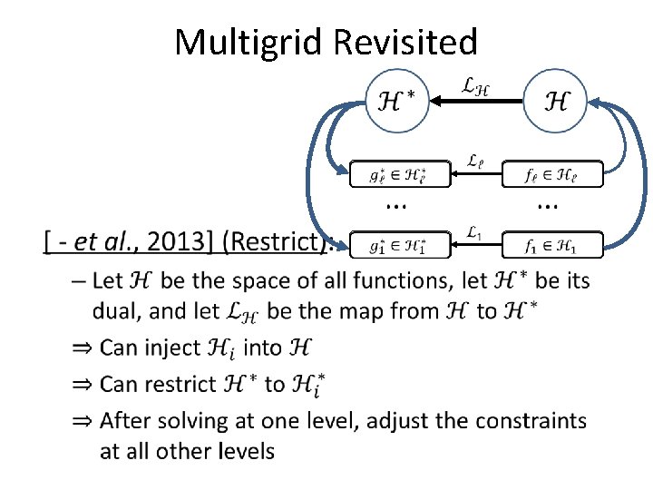
Multigrid Revisited •

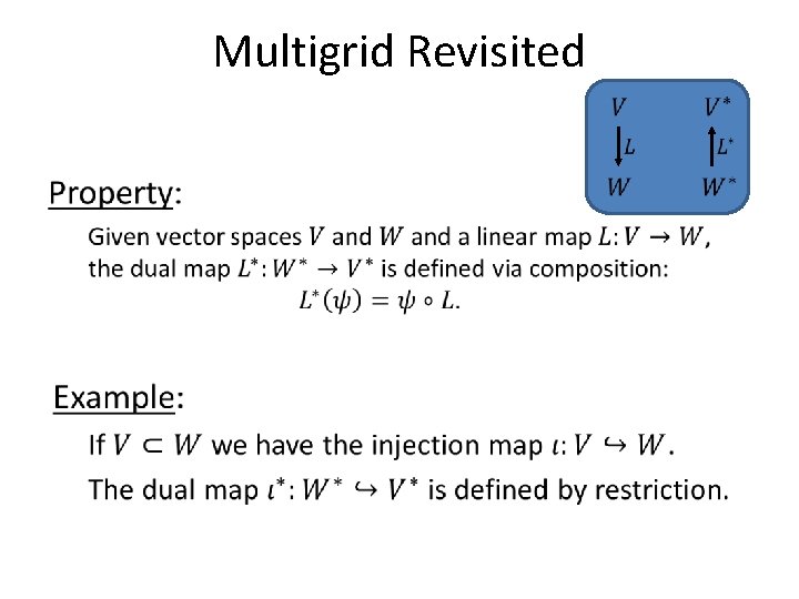
Multigrid Revisited •

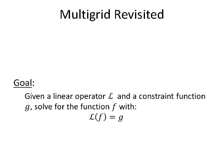
Multigrid Revisited •

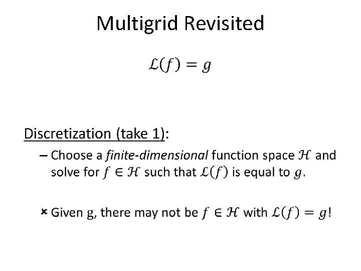
Multigrid Revisited •

Multigrid Revisited •

Multigrid Revisited •

Multigrid Revisited •

Multigrid Revisited •

Multigrid Revisited •

Multigrid Revisited •

Multigrid Revisited •

Multigrid Revisited [ - et al. , 2013] (Prolong): – Represent the solution as the sum of solutions from across levels Level 1 Level 2 Level 3 Level 4

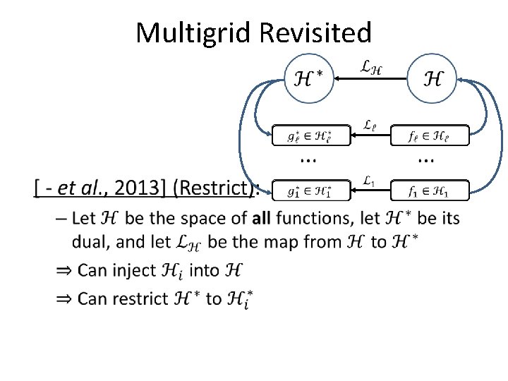
Multigrid Revisited •

Multigrid Revisited •

Multigrid Revisited [ - et al. , 2013]: Poisson reconstruction • • • Degree two B-splines Poisson equation Three dimensions CG relaxation Cascadic This work: Adaptive multigrid • • • Any degree B-splines Any (SPD) systems Any dimension GS relaxation V-Cycles

Outline • • • Motivation Multigrid Revisited Challenges Applications Conclusion

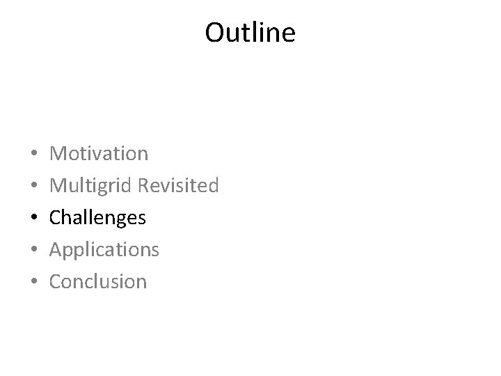
Challenges • Relax Down. Sample Up. Sample Solve level 1 level 2 level 3

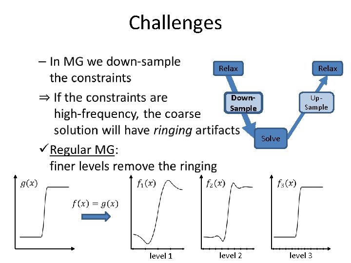
Challenges • Relax Down. Sample Up. Sample Solve level 2 level 3

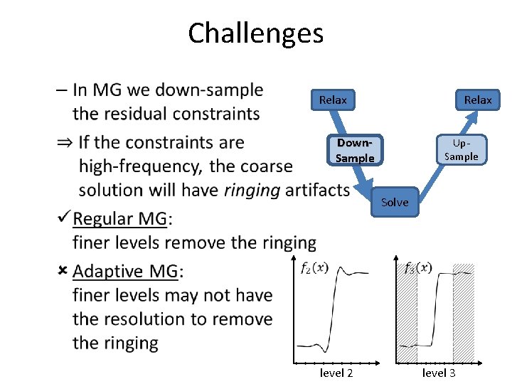
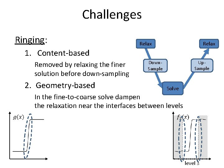
Challenges Ringing: Relax 1. Content-based Removed by relaxing the finer solution before down-sampling 2. Geometry-based Up. Sample Down. Sample Solve In the fine-to-coarse solve dampen the relaxation near the interfaces between levels level 3

Outline • • • Motivation Multigrid Revisited Challenges Applications Conclusion

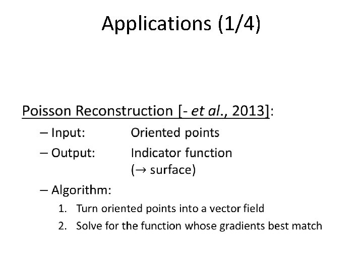
Applications (1/4) •

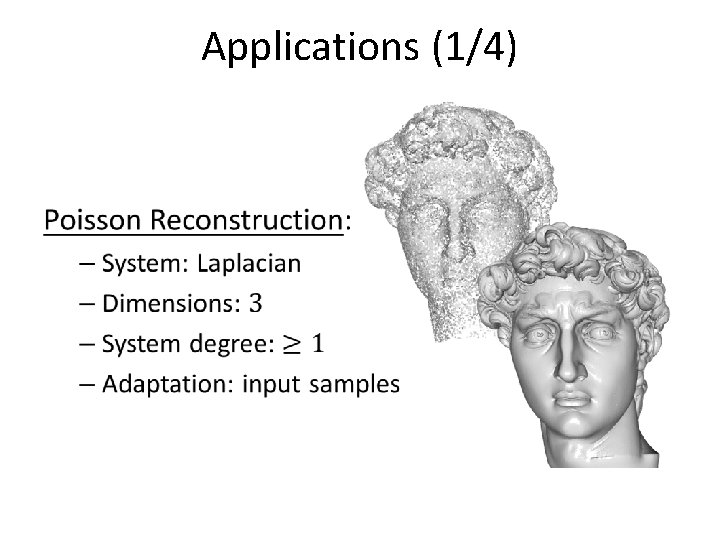
Applications (1/4) •

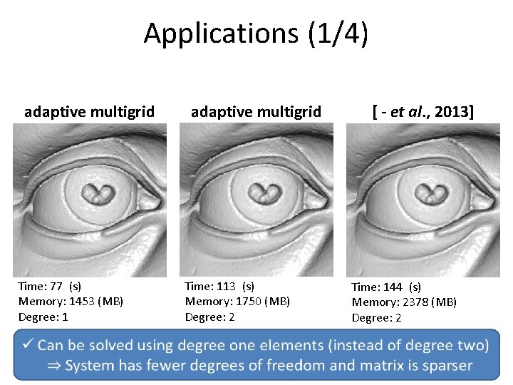
Applications (1/4) adaptive multigrid Time: 77 (s) Memory: 1453 (MB) Degree: 1 adaptive multigrid Time: 113 (s) Memory: 1750 (MB) Degree: 2 input points: 11 M resolution: 10243 [ - et al. , 2013] Time: 144 (s) Memory: 2378 (MB) Degree: 2

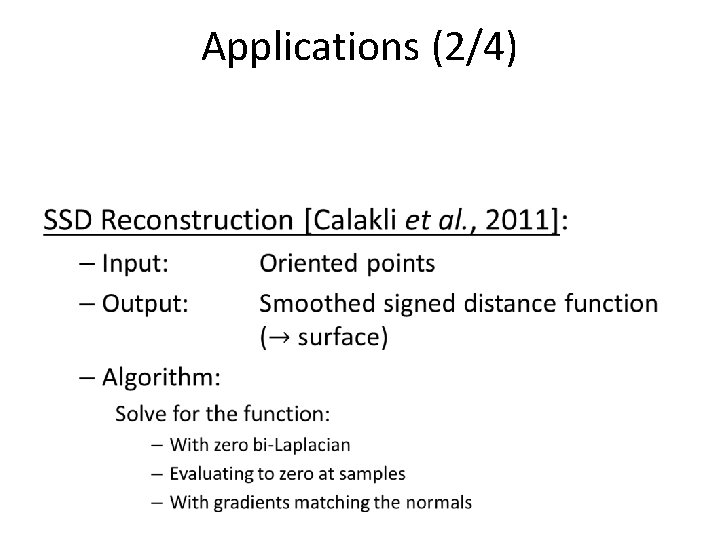
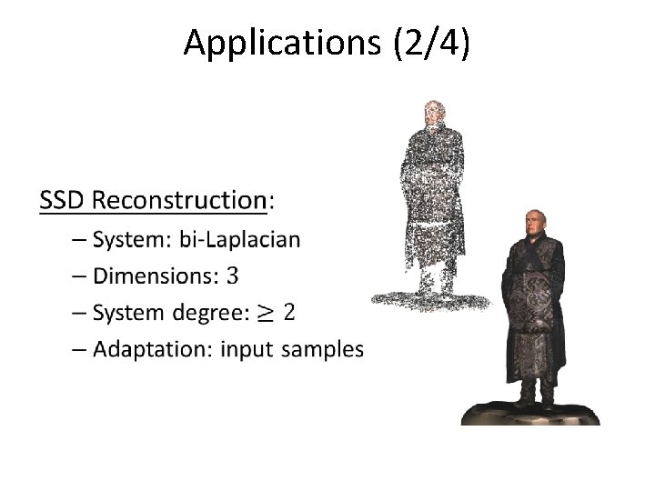
Applications (2/4) •

Applications (2/4) •

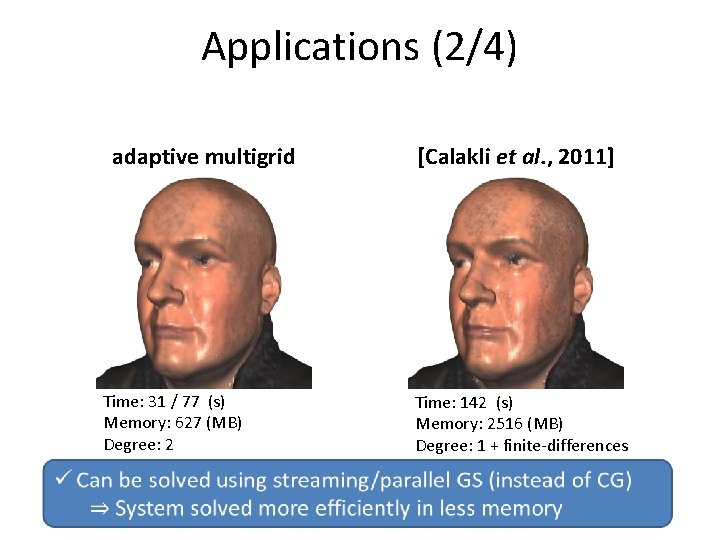
Applications (2/4) adaptive multigrid Time: 31 / 77 (s) Memory: 627 (MB) Degree: 2 [Calakli et al. , 2011] Time: 142 (s) Memory: 2516 (MB) Degree: 1 + finite-differences input points: 6 M resolution: 10243

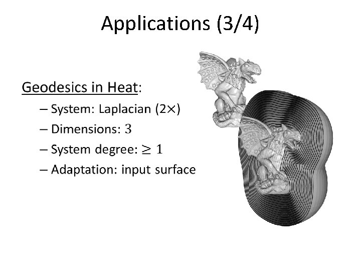
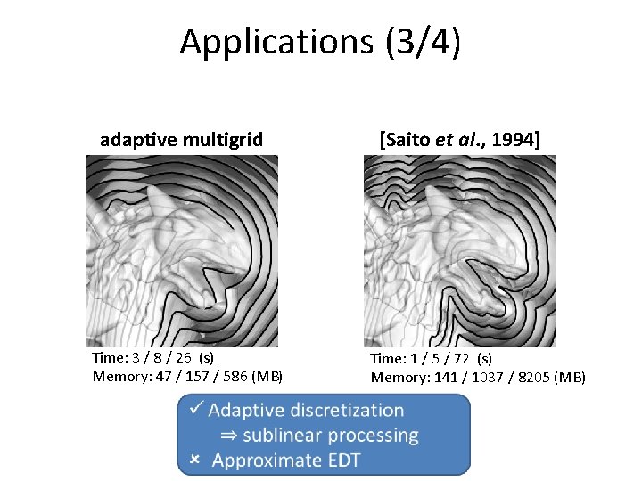
Applications (3/4) Geodesics in Heat [Crane et al. , 2013]: – Input: – Output: – Algorithm: Triangle mesh Unsigned distance function Solve for the function: – Diffuse a delta function of the mesh – Compute the (negated) gradient and normalize – Solve for the function whose gradients best match

Applications (3/4) •

Applications (3/4) adaptive multigrid Time: 3 / 8 / 26 (s) Memory: 47 / 157 / 586 (MB) [Saito et al. , 1994] Time: 1 / 5 / 72 (s) Memory: 141 / 1037 / 8205 (MB) input vertices: 214 K resolution: 2563 / 5123 / 10243

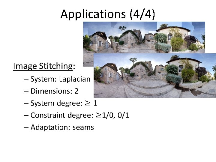
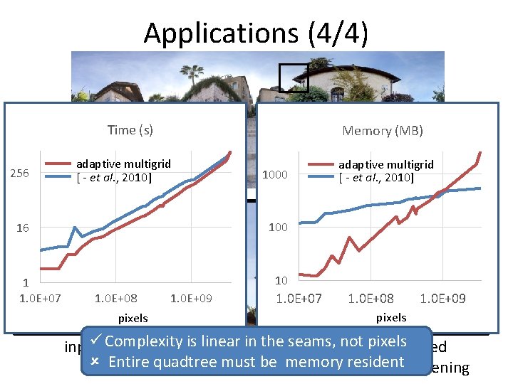
Applications (4/4) Image Stitching [Agarwala, 2007]: – Input: – Output: – Algorithm: Image composite Seamless panorama 1. Define a correction vector-field equal to – negative of the composite gradient across the seams – zero everywhere else 2. Solve for the function whose gradient best matches 3. Add the function to the composite

Applications (4/4) •

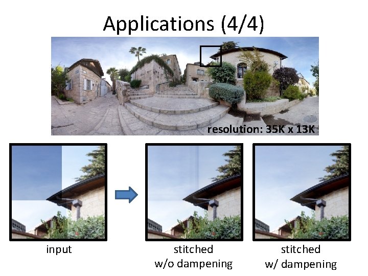
Applications (4/4) resolution: 35 K x 13 K input stitched w/o dampening stitched w/ dampening

Applications (4/4) Time (s) 256 Memory (MB) adaptive multigrid [ - et al. , 2010] 100 16 1 1. 0 E+07 1000 10 1. 0 E+08 pixels 1. 0 E+09 1. 0 E+07 1. 0 E+08 1. 0 E+09 pixels Complexity is linear in the seams, not pixels input stitched Entire quadtree must be memory resident w/o dampening w/ dampening

Conclusion Contribution: An adaptive multigrid solver supporting: – general degree elements – general SPD systems – general dimensions – etc.

Conclusion Future work: – Out-of-core – Improve ringing heuristic – Support boundary constraints

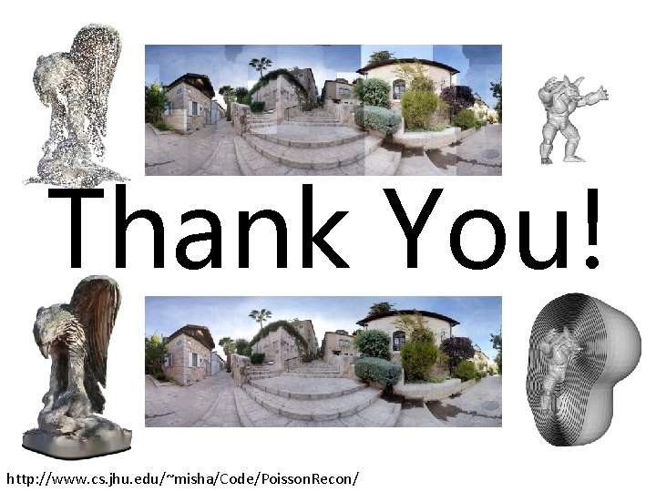
Thank You! http: //www. cs. jhu. edu/~misha/Code/Poisson. Recon/