AMS 345CSE 355 Computational Geometry Triangulation Algorithms Joe
![AMS 345/CSE 355 Computational Geometry Triangulation Algorithms Joe Mitchell Some figures: [O’Rourke]: Computational Geometry](https://slidetodoc.com/presentation_image_h/83d6cd500802c60fd3d7efe1c8be100c/image-1.jpg "AMS 345/CSE 355 Computational Geometry Triangulation Algorithms Joe Mitchell Some figures: [O’Rourke]: Computational Geometry")

 region bounded by")
![Simple Polygon n Definition in [O’Rourke]:](https://slidetodoc.com/presentation_image_h/83d6cd500802c60fd3d7efe1c8be100c/image-4.jpg "Simple Polygon n Definition in [O’Rourke]:")


![Diagonals [Devadoss-O’Rourke]](https://slidetodoc.com/presentation_image_h/83d6cd500802c60fd3d7efe1c8be100c/image-10.jpg "Diagonals [Devadoss-O’Rourke]")


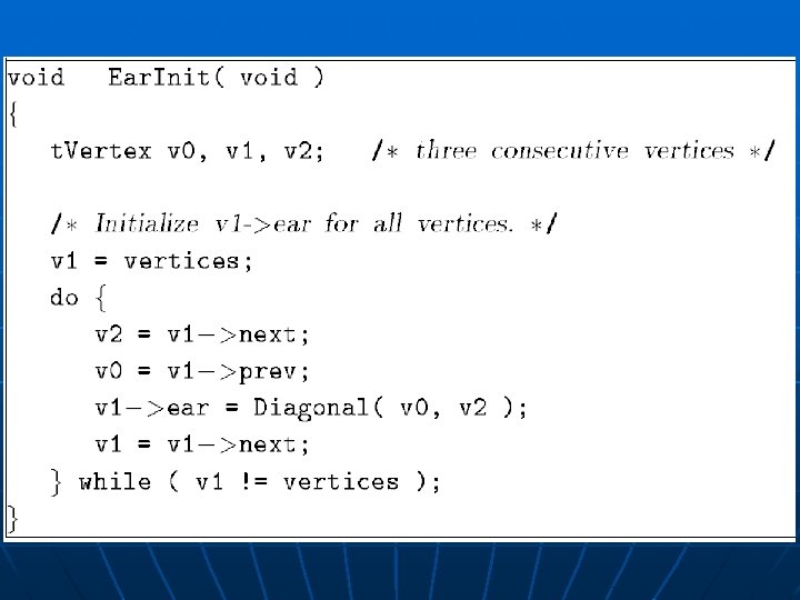
![Ears [Devadoss-O’Rourke] Proof(1): There are n edges of P and n-2 triangles in any](https://slidetodoc.com/presentation_image_h/83d6cd500802c60fd3d7efe1c8be100c/image-15.jpg "Ears [Devadoss-O’Rourke] Proof(1): There are n edges of P and n-2 triangles in any")
 Cases with")
 n n (n) : Have to read the data")


 Examples Exist")
 triangulation Examples Primitives: Left test, etc")
 n n n Input: PSLG of size n; enclosed")


 n Ear clipping is easy! • Testing if")
 38")

 n (1) Plane sweep to get horizontal trapezoidalization L")

 The “Sweep")


 updates to the SLS, each taking time")

 n (2) Join top vertex to bottom vertex in")
 n (3) Triangulate each monotone mountain Triangulate each, in")


,")


, using dynamic programming MWT")


- Slides: 67
AMS 345/CSE 355 Computational Geometry Triangulation Algorithms Joe Mitchell Some figures: [O’Rourke]: Computational Geometry in C: Chap 2
Triangulation n Input: Set S of n points n Input: Other shapes Simple polygon n Polygon with holes 3 D: Surfaces and solids (tetrahedralization) Planar Straight-Line Graph (PSLG) Triangulation applet for simple polygons 2
Simple Polygons n Definition: A simple polygon P is the (closed) region bounded by a “simple closed polygonal curve”.
Simple Polygon n Definition in [O’Rourke]:
Simple Polygons n Alternate Definition: P is a simple polygon if it is a simply connected (i. e. , no “holes”) subset of the plane whose boundary consists of a connected finite union of straight line segments.
Simple Polygons Some definitions would allow this as a “degenerate” simple polygon
Definitions: Visibility, Diagonals n For p, q in P, p is visible to q if segment pq lies within (closed) P p q
Definitions: Visibility, Diagonals n n For p, q in P, p is visible to q if segment pq lies within (closed) P p is clearly visible to q if p is visible to q AND the only points in common between pq and P are possibly p and q p clearly sees q but does not clearly see q’ p sees q’ p q q’
Definitions: Visibility, Diagonals n vivj is a diagonal if vi and vj are vertices that clearly see each other (versus: chord pq, with p and q on the boundary of P) q pq is a chord (not a diagonal) vivj is a diagonal vkvm is not a diagonal p vm vj vk vi
Diagonals [Devadoss-O’Rourke]
Triangulation n Definition: A partition of P into triangles by a set of noncrossing diagonals. (= a partition of P by a maximal set of noncrossing diagonals) [Devadoss-O’Rourke]
Triangulation Theory in 2 D n Also with holes Thm: A simple polygon has a triangulation. • Lem: An n-gon with n 4 has a diagonal. But, NOT true in 3 D! n n Thm: Any triangulation of a simple n-gon has n-3 diagonals, n-2 triangles. Thm: The “dual” graph is a tree. Thm: An n-gon with n 4 has 2 “ears”. Thm: The triangulation graph can be 3 -colored. Proofs: Induction on n. 12
Ears n n A diagonal of the form vi-1 vi+1 is an ear diagonal; the triangle vi-1 vivi+1 is an ear, and vi is the ear tip Note that there at most n ears (and that a convex polygon has exactly n ears) vi+1 vi-1 vi
Ears [Devadoss-O’Rourke] Proof(1): There are n edges of P and n-2 triangles in any triangulation. Imagine dropping the n edges into the n-2 “pigeonholes” corresponding to the triangles: Each edge appears on boundary of some triangle. By pigeonhole principle, at least 2 triangles get 2 edges “dropped in their box”. (2) Consider the planar dual (excluding the face at infinity) of a triangulation of P. Claim: The dual graph for a triangulated simple polygon is a TREE. Any tree of 2 or more nodes has at least 2 nodes of degree 1.
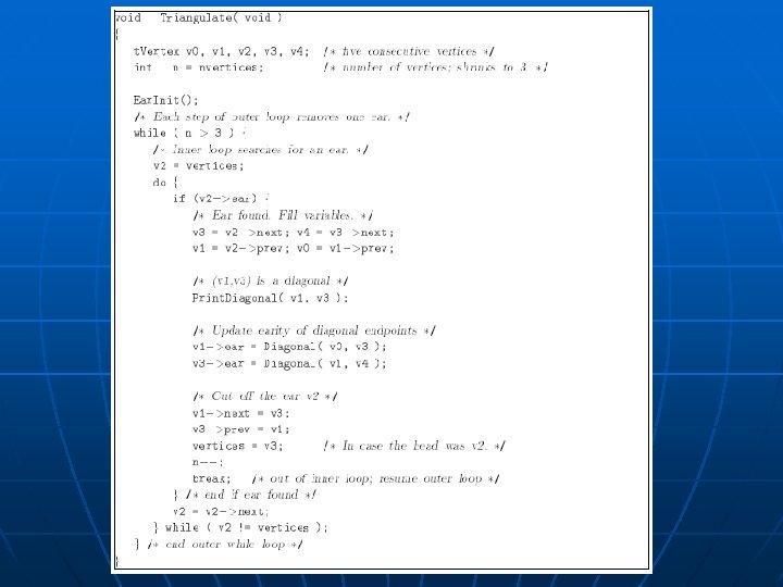
Triangulating a Simple Polygon n n Simple “ear-clipping” methods: O(n 2 ) Cases with simple O(n) algorithms: fan • Convex polygons (trivial!) • Monotone polygons, monotone mountains n General case (even with holes!): • Sweep algorithm to decompose into monotone mountains • O(n log n) n Best theoretical results: Not practical! • Simple polygons: O(n) [Chazelle’ 90] • Polygons with h holes: O(n+h log 1+ h), (n+h log h) [BC] n Good practical method: FIST [Held], based on clever methods of ear clipping (worst-case O(n 2 ) ) 16
Lower Bound (n+h log h) n n (n) : Have to read the data (h log h) : from SORTING 17
FIST: Fast Industrial-Strength Triangulation Based on ear clipping Simple polygon FIST Works nicely also for highly degenerate and “crazy” polygons Constrained Delaunay http: //www. cosy. sbg. ac. at/~held/projects/triang. html 3 D cycles
Ear-Clipping Triangulation Input: Simple polygon P vi+1 vi-1 vi pq is a diagonal, cutting off a single triangle (the “ear”) Naive: O(n 3) Smarter: Keep track of “ear tip status” of each vi (initialize: O(n 2) ) Each ear clip requires O(1) ear tip tests ( @ O(n) per test ) Thus, O(n 2) total, worst-case Ear-clipping applet
Triangulate
Ear-Clipping n Lemma: When clipping ear wth tip vi the only ear tip statuses that can change are at vi-1 and vi+1
Example: Triangulate
Example: Output
(n 2 ) Examples Exist
Today, 9/26/13 n n Review: O(n log n) triangulation Examples Primitives: Left test, etc Time permitting: Convex decompositions, Hertel-Mehlhorn
Faster Algorithm: O(n log n) n n n Input: PSLG of size n; enclosed by a big box B Step 1: Use sweep to decompose B into “y-monotone mountains” – y-monotone polygons having one side (left/right) a single segment (the “base”); O(n log n) Step 2: Triangulate each y-monotone polygon (size ni ) in time O(ni), for total O(n) Overall: O(n log n) to triangulate PSLG 28 n
Monotone Polygons n P is monotone in direction d t d b Every line perpendicular to d intersects P in a connected set; i. e. , the left/right chains from bottom, b, to top, t, are each d-monotone.
Monotone Polygons n P is monotone in direction d d
y-Monotone Polygon d
Examples n n Which of these polygons are monotone? (with respect to which directions d? ) Which are monotone mountains? With respect to which directions d?
Examples Circle of directions of monotonicity, d
Example from Practice Midterm
y-Monotone Polygon d
Monotone Mountains t d b
Triangulating a Monotone Mountain in O(n) n Ear clipping is easy! • Testing if vi-1 vi+1 is a diagonal takes t only O(1) time vi-1 vi vi+1 vi is ear tip iff Left(vi+1 , vi-1 ) Just traverse vertices from top to bottom. Test/clip ears. If an ear is clipped, re-test the earity of the upper endpoint (vi-1 ) of the diagonal just clipped. monotone 37 b
Triangulating a Monotone Mountain in O(n) 38
Example 39
Triangulation in O(n log n) n (1) Plane sweep to get horizontal trapezoidalization L Fire bullets left/right from each vertex SLS: left-to-right ordering of segments crossed by L (balanced binary 40 tree) Events: L hits a vertex Time: O(n log n)
Sweep Algorithms n Paradigm: Process geometric data by “sweeping” over it, in some order
Sweep Algorithms n Two key ingredients of any sweep algorithm: • (1) The “Sweep Line Status” (SLS): gives a “combinatorial description” of the “slice” given by the sweeping line n Often stored in a balanced binary tree • (2) Events: These are instants when the SLS “changes” combinatorially, and we must pause and do some event handling. Store in “Event Queue” (EQ), often a “priority queue” that allows us to quickly determine the next event n Often events occur at certain discrete points/vertices of the input; EQ is sometimes “static” (events known in advance), sometimes “dynamic” (events learned as we go)
Sweep Algorithms n What is needed to describe a sweep algorithm: • What is being “swept”? (line, plane, curve, etc) And how is it “sweeping”? (“order”? ) • What exactly does the SLS store, and in what kind of data structure is it stored (to provide for efficient updates as it changes)? • Exactly what are the “events”? How are they stored (the Event Queue, EQ)? How are they handled? Usually there are various cases, and one must specify for each exactly what updates are made to the SLS and the EQ (if any).
Trapezoidalization
Trapezoidalization
Trapezoidalization In each case: We do O(1) updates to the SLS, each taking time O(log n), since the SLS is stored in a balanced binary search tree.
Trapezoidalization
Triangulation in O(n log n) n (2) Join top vertex to bottom vertex in each trapezoid Lemma: Resulting pieces are monotone mountains 48
Triangulation in O(n log n) n (3) Triangulate each monotone mountain Triangulate each, in time O(ni ), for total time O(n) Summary: O(n log n) to triangulate n points or a planar straight-line graph (PSLG) 49
Bottom Line: Triangulation in 2 D n n Best theoretical results: • Simple polygons: O(n) [Chazelle’ 90] • Polygons with h holes: O(n+h log 1+ h), (n+h log h) [BC] • PSLG: for each simple face (without holes), O(ni); for each face with holes, O(ni+hi log 1+ hi) Good practical method: FIST [Held], based on clever methods of ear clipping (worst-case O(n 2 ))
Convex Decomposition n Partition simple polygon P into a small number of convex pieces One way to do it: Triangulate P
Convex Decomposition n Partition simple polygon P into a small number of convex pieces Another way to do it: Use diagonals to partition P into convex polygons
Convex Decomposition n Partition simple polygon P into a small number of convex pieces Another way to do it: Allow “Steiner” points (non-vertices) inside P. May get fewer pieces!
Convex Decomposition n Goal: Partition P into a small number of convex pieces (convex polygons) A triangulation is one possible decomposition into convex pieces, but it may have many more pieces than necessary! Dynamic Programming algorithms yield optimal solutions for simple polygons (for both Steiner and non-Steiner versions), in roughly O(n 3) O(r 2 n log n) without Steiner [Keil’ 85]; O(n+r 3) allowing Steiner [Chazelle’ 80] n Hertel-Mehlhorn algorithm: 4 -approximation in time O(n) 54
Convex Decomposition 55
Convex Decomposition 56
Optimal Convex Decomposition n Allowing Steiner points 57
Convex Decomposition r=6 58
Convex Decomposition One diagonal “resolves” the local nonconvexities at 2 reflex vertices at once We need at least r/2 segments to resolve all r reflex vertices Results in at least ceil(r/2)+1 pieces r=6 59
Hertel-Mehlhorn Algorithm n n Start with any triangulation of simple polygon P (time O(n), [Chazelle]) Remove inessential diagonals, in any order (time O(n), since we can test a diagonal locally in time O(1) to see if it is essential; if we remove a diagonal, we only have to update the “inessential” flag of O(1) other diagonals) 60
Hertel-Mehlhorn Algorithm n Lemma 2. 5. 2: At the end of the algorithm, for each reflex vertex v, there can be at most 2 diagonals essential for v 61
Hertel-Mehlhorn Algorithm n Theorem 2. 5. 3: The H-M algorithm yields a decomposition into at most 4*OPT pieces, where OPT is the minimum possible number of convex pieces in a (Steiner) convex decomposition. We say that the H-M Algorithm is a “ 4 -approximation algorithm” OPEN: Find a better factor than 4, which still runs very efficiently (say, in O(n log n) or O(n) time). 62
Hertel-Mehlhorn Algorithm n n n Proof: At end, each diagonal is essential for some (reflex) vertex. By Lemma 2. 5. 2, there at most 2 r diagonals left (since each reflex vertex is “responsible” for at most 2 diagonals) Thus, the number, M, of pieces is ≤ 2 r+1 < 2 r+4 ≤ 4*OPT (Since, by Theorem 2. 5. 1, OPT ≥ ceil(r/2)+1, so 4*OPT ≥ 4*ceil(r/2)+4≥ 2 r+4) 63
H-M Algorithm: Example
Minimum-Weight Triangulation n MWT of a simple polygon: O(n 3), using dynamic programming MWT of a polygon with holes (or of a set of points in the plane) is NP-hard Min-Weight Steiner Triangulation: allow extra “Steiner” points to be added AMS 545 / CSE 555 n n • Not known to exist • 316 -approximation known 65
MWT in Simple Polygon n n Dynamic Programming Bellman equation: AMS 545 / CSE 555 • Let f(i, j) be the total length of diagonals in a min-weight triangulation in the simple polygon left of diagonal (i, j). f(i, j) = 0, if (i, j) is ear diagonal; else, f(i, j)=mink: k sees i, j [|ik|+|kj|+f(i, k)+f(k, j)] k Time O(n 3) i j
Related Optimizations Using DP n n Min-max diagonal triangulation of P Max-min diagonal Min-max area triangle Max-min angle Min-max angle Fewest-guards-by-Fisk-method etc AMS 545 / CSE 555 n n n