Amortized Analysis Amortization Amortization is the paying off

Amortized Analysis

Amortization • Amortization is the paying off of debt with a fixed repayment schedule in regular instalments over a period of time for example with a mortgage or a car loan. • Amortization is a simple way to evenly spread out costs over a period of time. Typically, we amortize items such as loans, rent/mortgages, annual subscriptions

• The motivation for amortized analysis is that only looking at the worst-case run time per operation can be too pessimistic. • The technique was first formally introduced by Robert Tarjan in his 1985 paper Amortized Computational Complexity • Amortized analysis considers both the costly and less costly operations together over the whole series of operations of the algorithm. • Total cost of operations is evenly spread out across ‘n’ operations.

Incrementing a Binary Counter k-bit Binary Counter: A[0. . k 1] INCREMENT(A) 1. i 0 2. while i < length[A] and A[i] = 1 3. do A[i] 0 ⊳ reset a bit 4. i i+1 5. if i < length[A] 6. then A[i] 1 ⊳ set a bit

k-bit Binary Counter Ctr A[4] A[3] A[2] A[1] A[0] cost 0 0 0 1 1 2 0 0 1 0 3 3 0 0 1 1 4 4 0 0 0 7 5 0 1 1 0 1 8 6 0 1 1 0 10 7 0 1 11 8 1 0 0 0 15 9 1 0 0 1 16 10 1 0 18 11 1 0 1 1 19 12 1 1 0 0 22

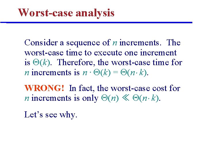
Worst-case analysis Consider a sequence of n increments. The worst-case time to execute one increment is (k). Therefore, the worst-case time for n increments is n · (k) = (n k). WRONG! In fact, the worst-case cost for n increments is only (n) ≪ (n k). Let’s see why.

Tighter analysis Ctr A[3] A[2] A[1] A[0] Cost Total cost of n operations 0 0 0 1 1 2 0 0 1 0 3 3 0 0 1 1 4 A[2] flipped every 4 ops n/22 4 0 1 0 0 7 A[3] flipped every 8 ops n/23 5 0 1 8 6 0 1 1 0 10 7 0 1 11 8 1 0 0 0 15 9 1 0 0 1 16 10 1 0 18 11 1 0 1 1 19 A[0] flipped every op n A[1] flipped every 2 ops n/2 … … A[i] flipped every 2 i ops … n/2 i

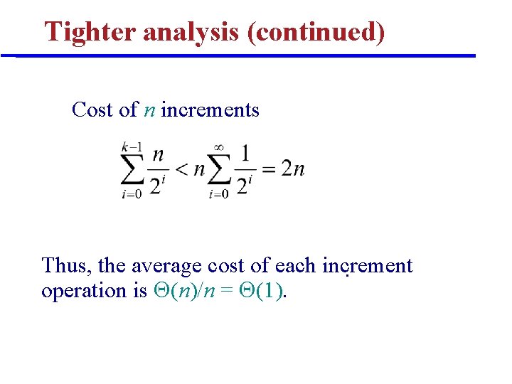
Tighter analysis (continued) Cost of n increments Thus, the average cost of each increment. operation is (n)/n = (1).

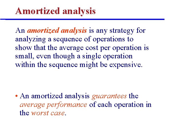
Amortized analysis An amortized analysis is any strategy for analyzing a sequence of operations to show that the average cost per operation is small, even though a single operation within the sequence might be expensive. • An amortized analysis guarantees the average performance of each operation in the worst case.

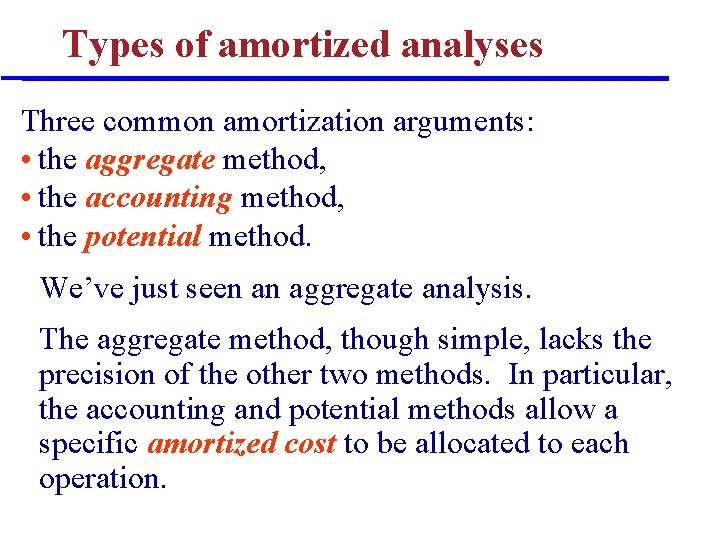
Types of amortized analyses Three common amortization arguments: • the aggregate method, • the accounting method, • the potential method. We’ve just seen an aggregate analysis. The aggregate method, though simple, lacks the precision of the other two methods. In particular, the accounting and potential methods allow a specific amortized cost to be allocated to each operation.

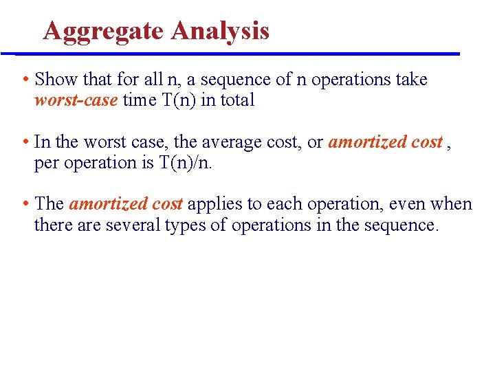
Aggregate Analysis • Show that for all n, a sequence of n operations take worst-case time T(n) in total • In the worst case, the average cost, or amortized cost , per operation is T(n)/n. • The amortized cost applies to each operation, even when there are several types of operations in the sequence.