Alternatives to Resolution IV Screening Designs in 16

Alternatives to Resolution IV Screening Designs in 16 Runs Douglas C. Montgomery Regents’ Professor of Industrial Engineering & Statistics ASU Foundation Professor of Engineering Arizona State University doug. montgomery@asu. edu No-Confounding Designs 1

Alternatives to Resolution IV Screening Designs in 16 Runs • This is joint work with Bradley Jones, SAS Institute • Jones, B. and Montgomery, D. C. (2010), “Alternatives to Resolution IV Screening Designs in 16 Runs”, International Journal of Experimental Design and Process Optimisation, Vol. 1, No. 4, pp. 285 -295. No-Confounding Designs 2

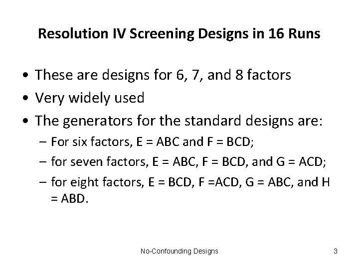
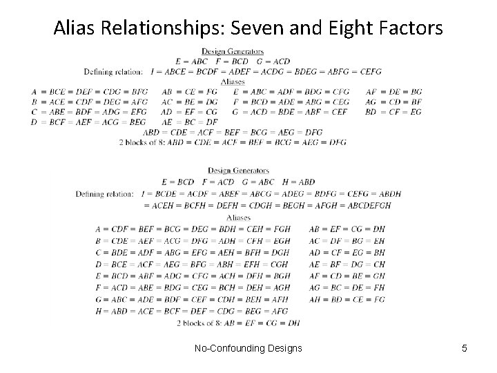
Resolution IV Screening Designs in 16 Runs • These are designs for 6, 7, and 8 factors • Very widely used • The generators for the standard designs are: – For six factors, E = ABC and F = BCD; – for seven factors, E = ABC, F = BCD, and G = ACD; – for eight factors, E = BCD, F =ACD, G = ABC, and H = ABD. No-Confounding Designs 3

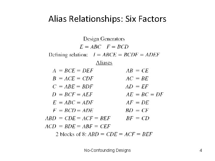
Alias Relationships: Six Factors No-Confounding Designs 4

Alias Relationships: Seven and Eight Factors No-Confounding Designs 5

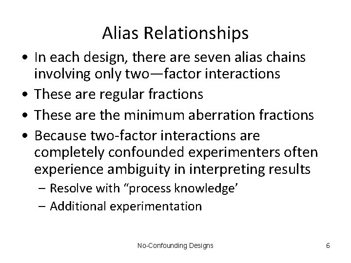
Alias Relationships • In each design, there are seven alias chains involving only two—factor interactions • These are regular fractions • These are the minimum aberration fractions • Because two-factor interactions are completely confounded experimenters often experience ambiguity in interpreting results – Resolve with “process knowledge’ – Additional experimentation No-Confounding Designs 6

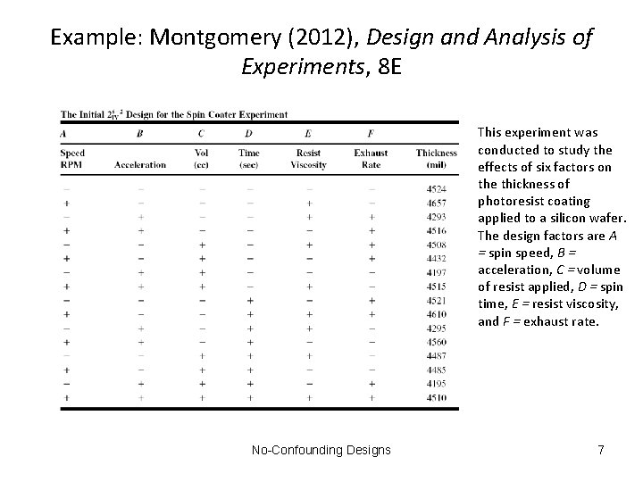
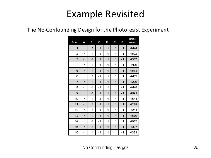
Example: Montgomery (2012), Design and Analysis of Experiments, 8 E This experiment was conducted to study the effects of six factors on the thickness of photoresist coating applied to a silicon wafer. The design factors are A = spin speed, B = acceleration, C = volume of resist applied, D = spin time, E = resist viscosity, and F = exhaust rate. No-Confounding Designs 7

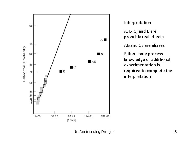
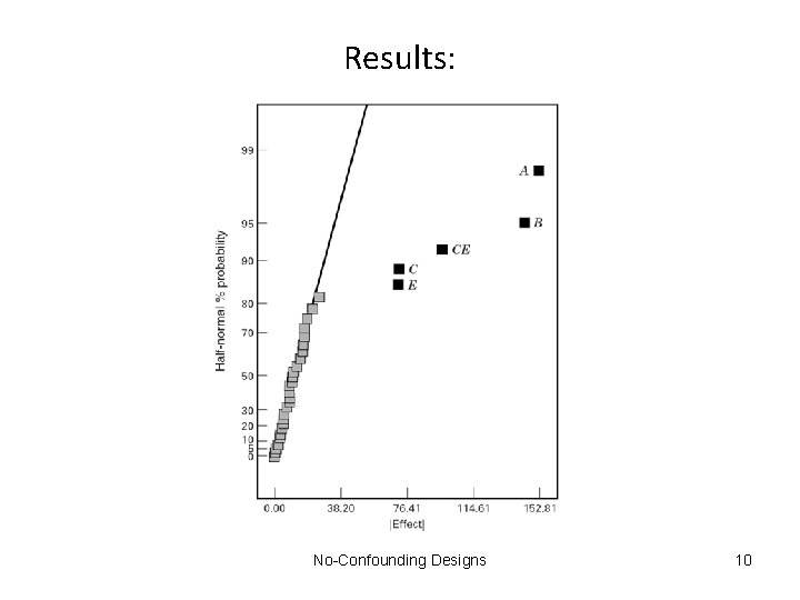
Interpretation: A, B, C, and E are probably real effects AB and CE are aliases Either some process knowledge or additional experimentation is required to complete the interpretation No-Confounding Designs 8

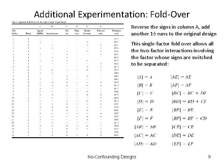
Additional Experimentation: Fold-Over Reverse the signs in column A, add another 16 runs to the original design This single-factor fold over allows all the two-factor interactions involving the factor whose signs are switched to be separated: No-Confounding Designs 9

Results: No-Confounding Designs 10

Other “Design Augmentation” Tricks • Partial fold-over, requiring only eight additional runs • Optimal augmentation (using the D-optimality criterion) • But what if additional experimentation isn’t an option? No-Confounding Designs 11

An Alternative to Additional Experimentation • While strong two-factor interactions may be less likely than strong main effects, there are many more interactions than main effects in screening situations. • It is not unusual to find that between 15 and 30% of the effects in a screening design are active • As a result, the likelihood of at least one significant interaction effect is high. • There is often substantial institutional reluctance to commit additional time and material (and sometimes it’s impossible). Consequently, experimenters would like to avoid the need for a follow-up study. • We show can lower the risk of analytical ambiguity by using a specific orthogonal but non-regular fractional factorial design. • The proposed designs for six, seven, and eight factor studies in 16 runs have no complete confounding of pairs of two-factor interactions. No-Confounding Designs 12

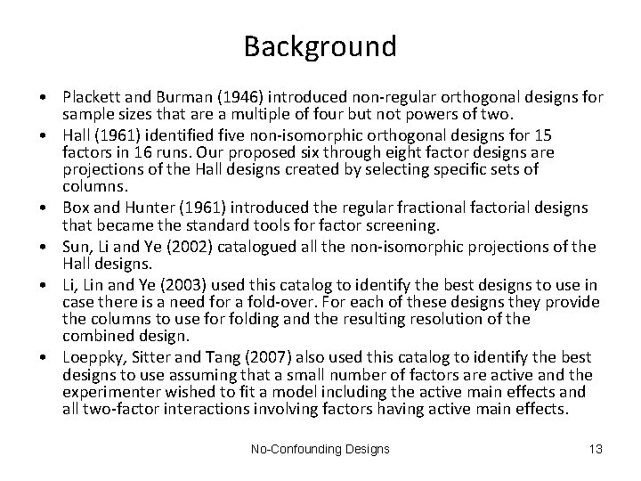
Background • Plackett and Burman (1946) introduced non-regular orthogonal designs for sample sizes that are a multiple of four but not powers of two. • Hall (1961) identified five non-isomorphic orthogonal designs for 15 factors in 16 runs. Our proposed six through eight factor designs are projections of the Hall designs created by selecting specific sets of columns. • Box and Hunter (1961) introduced the regular fractional factorial designs that became the standard tools for factor screening. • Sun, Li and Ye (2002) catalogued all the non-isomorphic projections of the Hall designs. • Li, Lin and Ye (2003) used this catalog to identify the best designs to use in case there is a need for a fold-over. For each of these designs they provide the columns to use for folding and the resulting resolution of the combined design. • Loeppky, Sitter and Tang (2007) also used this catalog to identify the best designs to use assuming that a small number of factors are active and the experimenter wished to fit a model including the active main effects and all two-factor interactions involving factors having active main effects. No-Confounding Designs 13

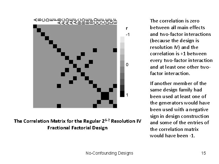
Metrics for Comparing Screening Designs Consider the model y=Xβ+e where X contains columns for the intercept, main effects and all two-factor interactions, β is the vector of model parameters, and ε is the usual error vector. For six through eight factors in 16 runs, the matrix, X, has more columns than rows. Thus, it is not of full rank and the usual least squares estimate for β does not exist because the matrix X’X is singular. With respect to this model, every 16 run design is supersaturated. Booth and Cox (1962) introduced the E(s 2) criterion as a diagnostic measure for comparing supersaturated designs: Minimizing the E(s 2) criterion is equivalent to minimizing the sum of squared off-diagonal elements of the correlation matrix of X. No-Confounding Designs 14

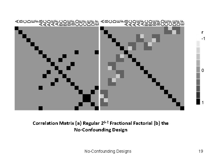
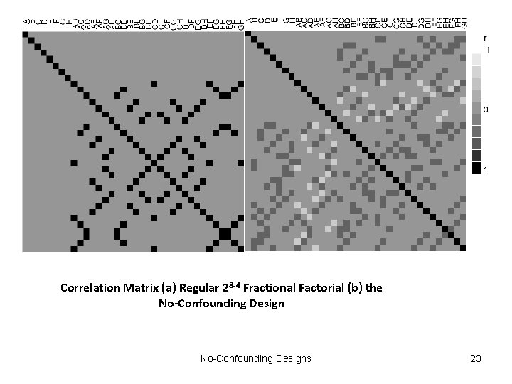
The correlation is zero between all main effects and two-factor interactions (because the design is resolution IV) and the correlation is +1 between every two-factor interaction and at least one other twofactor interaction. The Correlation Matrix for the Regular 26 -2 Resolution IV Fractional Factorial Design No-Confounding Designs If another member of the same design family had been used at least one of the generators would have been used with a negative sign in design construction and some of the entries of the correlation matrix would have been -1. 15

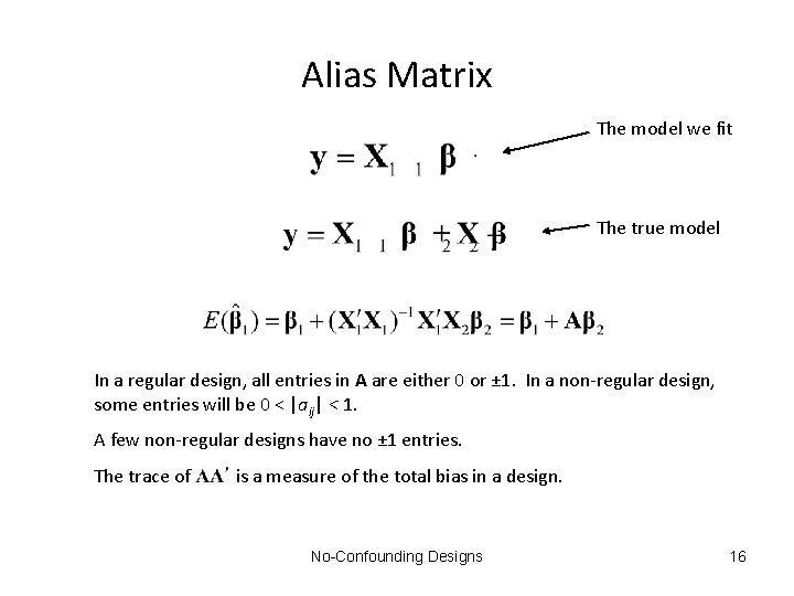
Alias Matrix The model we fit The true model In a regular design, all entries in A are either 0 or ± 1. In a non-regular design, some entries will be 0 < |aij| < 1. A few non-regular designs have no ± 1 entries. The trace of is a measure of the total bias in a design. No-Confounding Designs 16

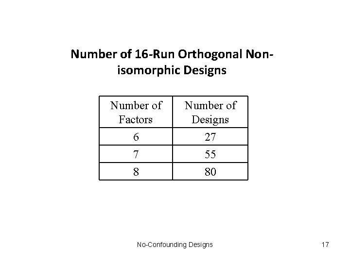
Number of 16 -Run Orthogonal Nonisomorphic Designs Number of Factors 6 7 Number of Designs 27 55 8 80 No-Confounding Designs 17

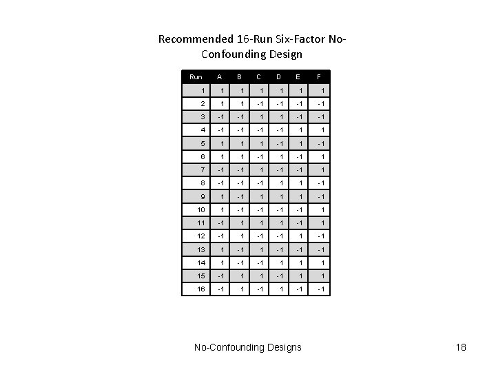
Recommended 16 -Run Six-Factor No. Confounding Design Run A B C D E F 1 1 1 1 2 1 1 -1 -1 3 -1 -1 1 1 -1 -1 4 -1 -1 1 1 5 1 1 1 -1 6 1 1 -1 1 7 -1 -1 1 8 -1 -1 -1 1 1 -1 9 1 -1 10 1 -1 -1 1 11 -1 1 12 -1 13 1 -1 -1 -1 14 1 -1 -1 1 15 -1 1 1 16 -1 1 -1 -1 No-Confounding Designs 18

Correlation Matrix (a) Regular 26 -2 Fractional Factorial (b) the No-Confounding Designs 19

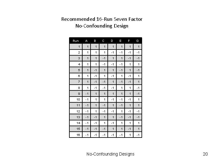
Recommended 16 -Run Seven Factor No-Confounding Design Run A B C D E F G 1 1 1 1 2 1 1 1 -1 -1 3 1 1 -1 -1 4 1 1 -1 -1 -1 1 1 5 1 -1 6 1 -1 1 7 1 -1 -1 1 8 1 -1 -1 -1 1 1 -1 9 -1 1 1 -1 10 -1 1 1 -1 -1 -1 1 11 -1 1 1 12 -1 1 -1 -1 13 -1 -1 1 1 -1 -1 -1 14 -1 -1 1 1 1 15 -1 -1 -1 1 16 -1 -1 -1 No-Confounding Designs 20

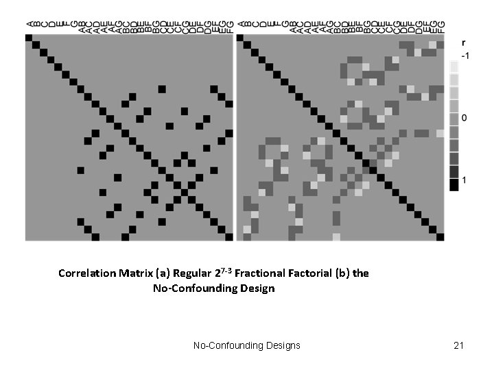
Correlation Matrix (a) Regular 27 -3 Fractional Factorial (b) the No-Confounding Designs 21

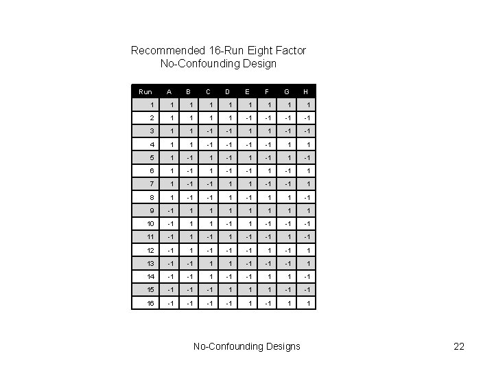
Recommended 16 -Run Eight Factor No-Confounding Design Run A B C D E F G H 1 1 1 1 1 2 1 1 -1 -1 3 1 1 -1 -1 4 1 1 -1 -1 1 1 5 1 -1 6 1 -1 -1 1 7 1 -1 -1 1 8 1 -1 -1 1 1 -1 9 -1 1 1 1 10 -1 1 1 -1 -1 -1 1 -1 12 -1 1 -1 -1 -1 1 13 -1 -1 1 1 -1 -1 -1 1 14 -1 -1 15 -1 -1 -1 16 -1 -1 1 1 No-Confounding Designs 22

Correlation Matrix (a) Regular 28 -4 Fractional Factorial (b) the No-Confounding Designs 23

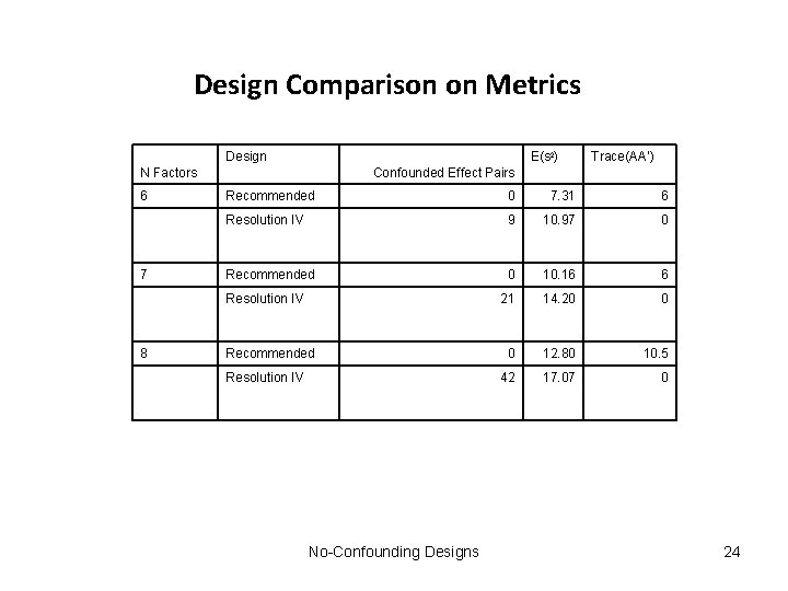
Design Comparison on Metrics Design E(s 2) N Factors 6 7 Confounded Effect Pairs Recommended 0 7. 31 6 Resolution IV 9 10. 97 0 Recommended 0 10. 16 6 21 14. 20 0 0 12. 80 10. 5 42 17. 07 0 Resolution IV 8 Trace(AA’) Recommended Resolution IV No-Confounding Designs 24

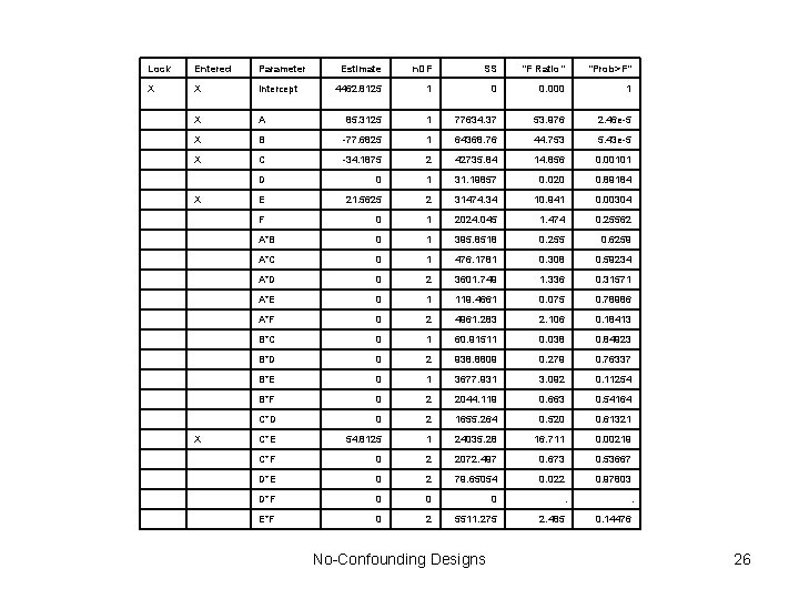
Example Revisited The No-Confounding Design for the Photoresist Experiment Run A B C D E F Thick ness 1 1 1 1 4494 2 1 1 -1 -1 4592 3 -1 -1 1 1 -1 -1 4357 4 -1 -1 1 1 4489 5 1 1 1 -1 4513 6 1 1 -1 1 4483 7 -1 -1 1 4288 8 -1 -1 -1 1 1 -1 4448 9 1 -1 4691 10 1 -1 -1 1 4671 11 -1 1 4219 12 -1 1 -1 4271 13 1 -1 -1 -1 4530 14 1 -1 -1 1 4632 15 -1 1 1 4337 16 -1 1 -1 -1 4391 No-Confounding Designs 25

Lock Entered Parameter Estimate n. DF SS "F Ratio" "Prob>F" X X Intercept 4462. 8125 1 0 0. 000 1 X A 85. 3125 1 77634. 37 53. 976 2. 46 e-5 X B -77. 6825 1 64368. 76 44. 753 5. 43 e-5 X C -34. 1875 2 42735. 84 14. 856 0. 00101 D 0 1 31. 19857 0. 020 0. 89184 E 21. 5625 2 31474. 34 10. 941 0. 00304 F 0 1 2024. 045 1. 474 0. 25562 A*B 0 1 395. 8518 0. 255 0. 6259 A*C 0 1 476. 1781 0. 308 0. 59234 A*D 0 2 3601. 749 1. 336 0. 31571 A*E 0 1 119. 4661 0. 075 0. 78986 A*F 0 2 4961. 283 2. 106 0. 18413 B*C 0 1 60. 91511 0. 038 0. 84923 B*D 0 2 938. 8809 0. 279 0. 76337 B*E 0 1 3677. 931 3. 092 0. 11254 B*F 0 2 2044. 119 0. 663 0. 54164 C*D 0 2 1655. 264 0. 520 0. 61321 C*E 54. 8125 1 24035. 28 16. 711 0. 00219 C*F 0 2 2072. 497 0. 673 0. 53667 D*E 0 2 79. 65054 0. 022 0. 97803 D*F 0 0 0 . . E*F 0 2 5511. 275 2. 485 0. 14476 X X No-Confounding Designs 26

If I only knew then what I know now… No-Confounding Designs 27

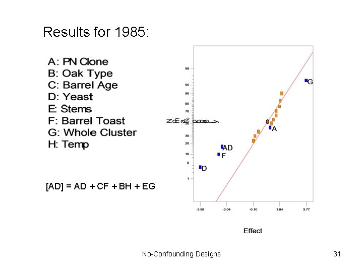
A personal experience with DOX: Wine-making. Original vineyard property purchased in 1983. Objectives were to begin as a grape supplier to other winemakers, then develop a winemaking process. Big problem: none of the partners were winemakers (how do you make a small fortune in wine…”). However, some partners knew the power of designed experiments. “Wine-making is a chemical process…I didn’t know how to make polymer, either, when I took my first job as a chemical engineer. ” No-Confounding Designs 28

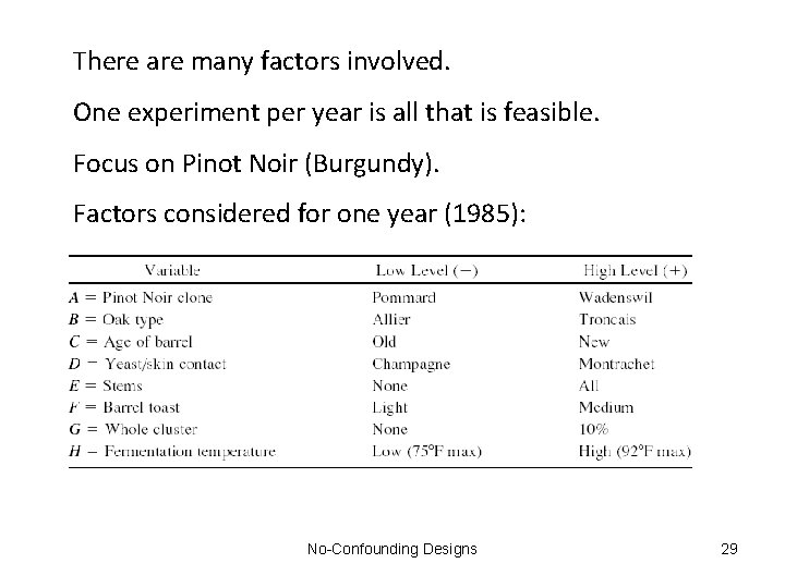
There are many factors involved. One experiment per year is all that is feasible. Focus on Pinot Noir (Burgundy). Factors considered for one year (1985): No-Confounding Designs 29

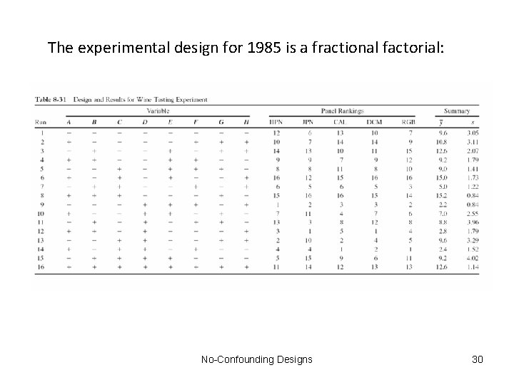
The experimental design for 1985 is a fractional factorial: No-Confounding Designs 30

Results for 1985: [AD] = AD + CF + BH + EG No-Confounding Designs 31

Some of the results are interesting and useful, such as 1. toasting the barrel a little more seems like a good idea, and 2. it doesn’t seem to matter much where the oak comes from. Some results are surprising such as no temperature effect! There is an interaction: [AD] = AD + CF + BH + EG Which effect(s) are real? CF and EG are more intuitive than AD, but we really don’t have any “process knowledge” How would we normally resolve this? 1. Fold-over (be careful)? 2. Partial fold-over? 3. Would the recommended non-regular designs have been better? No-Confounding Designs 32

How did we do? First commercial release, the 1990 Pinot Noir, won a gold medal at the American Wine Competition 1991 release won a silver medal 1992 release won gold a medal, sixth best wine overall (of 2000 entries), best Oregon Pinot Noir Consistently ranked by The Wine Spectator as among the best Pinot Noir available, 91 -94 rating Consistently highly rated in the International Pinot Noir Competition No-Confounding Designs 33

No-Confounding Designs 34

Other Work • What’s the power of these designs? • How many two-factor interactions can we detect? • Projections? • Analysis methods? • What about the resolution III case (9 -15 factors in 16 runs)? No-Confounding Designs 35

References • • • Booth, K. H. V. , Cox, D. R. , (1962). “Some systematic supersaturated designs. ” Technometrics 4, 489– 495. Box, G. E. P. and Hunter, J. S. (1961). “The 2 k-p Fractional Factorial Designs. ” Technometrics 3, pp. 449– 458. Bursztyn, D. and Steinberg, D. (2006). “Comparison of designs for computer experiments” Journal of Statistical Planning and Inference 136, pp. 1103 -1119. Hall, M. Jr. (1961). Hadamard matrix of order 16. Jet Propulsion Laboratory Research Summary, 1, pp. 21– 26. Jones, B. and Montgomery, D. C. (2010), “Alternatives to Resolution IV Screening Designs in 16 Runs”, International Journal of Experimental Design and Process Optimisation, Vol. 1, No. 4, pp. 285 -295. Li, W. , Lin, D. K. J. , Ye, K. (2003) “Optimal Foldover Plans for Two-Level Non-regular Orthogonal Designs” Technometrics 45, pp. 347– 351. Plackett, R. L. and Burman, J. P. (1946). “The Design of Optimum Multifactor Experiments. ” Biometrika 33, pp. 305– 325. Loeppky, J. L. , Sitter, R. R. , and Tang, B. (2007) “Nonregular Designs With Desirable Projection Properties. ” Technometrics 49, pp. 454– 466. Montgomery, D. C. (2009). Design and Analysis of Experiments 7 th Edition. Wiley Hoboken, New Jersey. Sun, D. X. , Li, W. , and Ye, K. Q. (2002). “An Algorithm for Sequentially Constructing Non. Isomorphic Orthogonal Designs and Its Applications. ” Technical Report SUNYSB-AMS-02 -13, State University of New York at Stony Brook, Dept. of Applied Mathematics and Statistics. No-Confounding Designs 36