Alpha Diversity Indices James A DanoffBurg Dept Ecol

Alpha Diversity Indices James A. Danoff-Burg Dept. Ecol. , Evol. , & Envir. Biol. Columbia University

Alpha Diversity Indices Q-Statistic Intro to Alpha Diversity Indices Simpson Mc. Intosh Berger-Parker Shannon-Wiener Brillouin Jack-Knifing Diversity Indices Pielou’s Hierarchical Diversity Index Lecture 4 – Alpha Diversity Indices Week 1 Week 2 © 2003 Dr. James A. Danoff-Burg, jd 363@columbia. edu

Diversity of Diversities Difference between the diversities is usually one of relative emphasis of two main envir. aspects Two key features þ þ Richness Abundance – our emphasis today Each index differs in the mathematical method of relating these features þ þ One is often given greater prominence than the other Formulae significantly differ between indices Lecture 4 – Alpha Diversity Indices © 2003 Dr. James A. Danoff-Burg, jd 363@columbia. edu

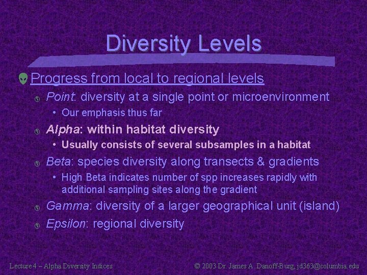
Diversity Levels Progress from local to regional levels þ Point: diversity at a single point or microenvironment • Our emphasis thus far þ Alpha: within habitat diversity • Usually consists of several subsamples in a habitat þ Beta: species diversity along transects & gradients • High Beta indicates number of spp increases rapidly with additional sampling sites along the gradient þ þ Gamma: diversity of a larger geographical unit (island) Epsilon: regional diversity Lecture 4 – Alpha Diversity Indices © 2003 Dr. James A. Danoff-Burg, jd 363@columbia. edu

Q Statistic Introduction A bridge between the abundance models & diversity indices þ Does not involve fitting a model • as in the abundance models Provides an indication of community diversity þ No weighting towards very abundant or rare species • They are excluded from the analysis • Whittaker (1972) created earlier analysis including these – Thereby more influenced by the few rare / abundant species þ Proposed by Kempton & Taylor (1976) Lecture 4 – Alpha Diversity Indices © 2003 Dr. James A. Danoff-Burg, jd 363@columbia. edu

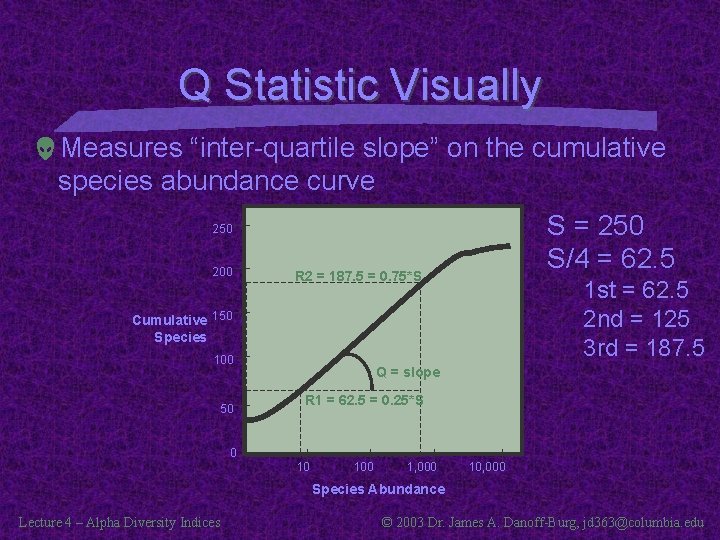
Q Statistic Visually Measures “inter-quartile slope” on the cumulative species abundance curve S = 250 S/4 = 62. 5 250 200 R 2 = 187. 5 = 0. 75*S 1 st = 62. 5 2 nd = 125 3 rd = 187. 5 Cumulative 150 Species 100 50 Q = slope R 1 = 62. 5 = 0. 25*S 0 10 100 1, 000 10, 000 Species Abundance Lecture 4 – Alpha Diversity Indices © 2003 Dr. James A. Danoff-Burg, jd 363@columbia. edu

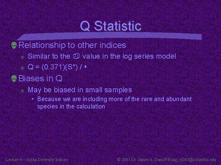
Q Statistic Relationship to other indices þ þ Similar to the a value in the log series model Q = (0. 371)(S*) / s Biases in Q þ May be biased in small samples • Because we are including more of the rare and abundant species in the calculation Lecture 4 – Alpha Diversity Indices © 2003 Dr. James A. Danoff-Burg, jd 363@columbia. edu

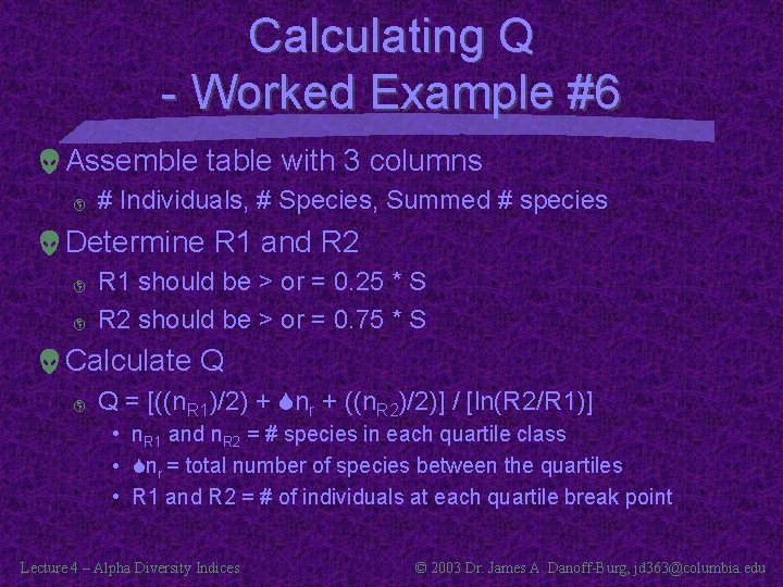
Calculating Q - Worked Example #6 Assemble table with 3 columns þ # Individuals, # Species, Summed # species Determine R 1 and R 2 þ þ R 1 should be > or = 0. 25 * S R 2 should be > or = 0. 75 * S Calculate Q þ Q = [((n. R 1)/2) + Snr + ((n. R 2)/2)] / [ln(R 2/R 1)] • n. R 1 and n. R 2 = # species in each quartile class • Snr = total number of species between the quartiles • R 1 and R 2 = # of individuals at each quartile break point Lecture 4 – Alpha Diversity Indices © 2003 Dr. James A. Danoff-Burg, jd 363@columbia. edu

Alpha Diversity Indices Q-Statistic Intro to Alpha Diversity Indices Simpson Mc. Intosh Berger-Parker Shannon-Wiener Brillouin Jack-Knifing Diversity Indices Pielou’s Hierarchical Diversity Index Lecture 4 – Alpha Diversity Indices Week 1 Week 2 © 2003 Dr. James A. Danoff-Burg, jd 363@columbia. edu

Alpha Diversity Indices All based on proportional species abundances þ Species abundance models have drawbacks • Tedious and repetitive • Problems if the data do not violate more than one model – How to choose between? Building upon the species abundance models þ Allows formal comparisons between sites / treatments Lecture 4 – Alpha Diversity Indices © 2003 Dr. James A. Danoff-Burg, jd 363@columbia. edu

Alpha Diversity Indices “Heterogeneity Indices” þ þ Consider both evenness AND richness Species abundance models only consider evenness No assumptions made about species abundance distributions þ þ Cause of distribution Shape of curve “Non-parametric” þ Free of assumptions of normality Lecture 4 – Alpha Diversity Indices © 2003 Dr. James A. Danoff-Burg, jd 363@columbia. edu

Two General Categories Information Theory (complicated computation) þ þ Diversity (or information) of a natural system is similar to info in a code or message Examples: Shannon-Wiener and Brillouin Indices Species Dominance Measures (simple comput. ) þ þ þ Weighted towards abundance of the commonest species Total species richness is downweighted relative to evenness Examples: Simpson, Mc. Intosh, and Berger-Parker Lecture 4 – Alpha Diversity Indices © 2003 Dr. James A. Danoff-Burg, jd 363@columbia. edu

Alpha Diversity Indices Q-Statistic Intro to Alpha Diversity Indices Simpson Mc. Intosh Berger-Parker Shannon-Wiener Brillouin Jack-Knifing Diversity Indices Pielou’s Hierarchical Diversity Index Lecture 4 – Alpha Diversity Indices Week 1 Week 2 © 2003 Dr. James A. Danoff-Burg, jd 363@columbia. edu

Simpson Index Values Derived by Simpson (1949) Basis þ þ Probability of 2 individuals being conspecifics If drawn randomly from an infinitely large community Summarized by letter D, 1 -D, or 1/D þ D decreases with increasing diversity • Can go from 1 – 30+ • Probability that two species are conspecifics with diversity þ 1 -D and 1/D increases with increasing diversity • 0. 0 < 1 -D < 1. 0 • 0. 0 < 1/D < 10+ Lecture 4 – Alpha Diversity Indices © 2003 Dr. James A. Danoff-Burg, jd 363@columbia. edu

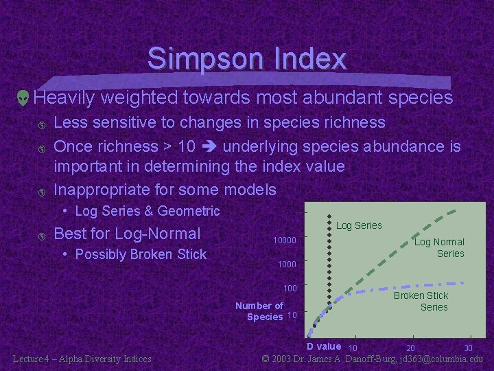
Simpson Index Heavily weighted towards most abundant species þ þ þ Less sensitive to changes in species richness Once richness > 10 underlying species abundance is important in determining the index value Inappropriate for some models • Log Series & Geometric þ Best for Log-Normal • Possibly Broken Stick Log Series 10000 100 Number of Species 10 Lecture 4 – Alpha Diversity Indices Log Normal Series Broken Stick Series D value 10 20 30 © 2003 Dr. James A. Danoff-Burg, jd 363@columbia. edu

Simpson Index When would this weight towards most abundant species be desired? þ Not just when the abundance model fits the Log-Normal Conservation implications of index use? Lecture 4 – Alpha Diversity Indices © 2003 Dr. James A. Danoff-Burg, jd 363@columbia. edu

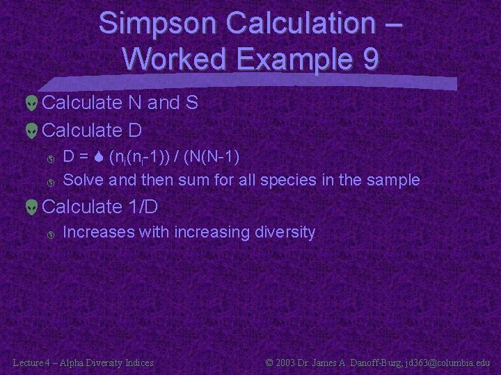
Simpson Calculation – Worked Example 9 Calculate N and S Calculate D þ þ D = S (ni(ni-1)) / (N(N-1) Solve and then sum for all species in the sample Calculate 1/D þ Increases with increasing diversity Lecture 4 – Alpha Diversity Indices © 2003 Dr. James A. Danoff-Burg, jd 363@columbia. edu

Alpha Diversity Indices Q-Statistic Intro to Alpha Diversity Indices Simpson Mc. Intosh Berger-Parker Shannon-Wiener Brillouin Jack-Knifing Diversity Indices Pielou’s Hierarchical Diversity Index Lecture 4 – Alpha Diversity Indices Week 1 Week 2 © 2003 Dr. James A. Danoff-Burg, jd 363@columbia. edu

Mc. Intosh Index Proposed by Mc. Intosh (1967) Community is a point in an S dimensional hypervolume whose Euclidean distance from the origin is a measure of diversity þ þ Paraphrased from Magurran Origin is no diversity, distances from origin are more diverse Not strictly a dominance index þ Needs conversion to dominance index Lecture 4 – Alpha Diversity Indices © 2003 Dr. James A. Danoff-Burg, jd 363@columbia. edu

Mc. Intosh Manipulations Base calculations (U metric) þ Strongly influenced by sample size Conversion to a dominance measure (D) þ þ Use Dm for our class Makes value independent of sample size Derive a simple evenness index using Mc. Intosh þ Most often used contribution of Mc. Intosh Lecture 4 – Alpha Diversity Indices © 2003 Dr. James A. Danoff-Burg, jd 363@columbia. edu

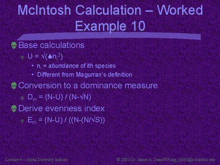
Mc. Intosh Calculation – Worked Example 10 Base calculations þ U = (Sni 2) • ni = abundance of ith species • Different from Magurran’s definition Conversion to a dominance measure þ Dm = (N-U) / (N- N) Derive evenness index þ Em = (N-U) / ((N-(N/ S)) Lecture 4 – Alpha Diversity Indices © 2003 Dr. James A. Danoff-Burg, jd 363@columbia. edu

Alpha Diversity Indices Q-Statistic Intro to Alpha Diversity Indices Simpson Mc. Intosh Berger-Parker Shannon-Wiener Brillouin Jack-Knifing Diversity Indices Pielou’s Hierarchical Diversity Index Lecture 4 – Alpha Diversity Indices Week 1 Week 2 © 2003 Dr. James A. Danoff-Burg, jd 363@columbia. edu

Berger-Parker Proposed by Berger and Parker (1970) and developed by May (1975) Simple calculation = d Expresses proportional importance of most abundant species Lecture 4 – Alpha Diversity Indices © 2003 Dr. James A. Danoff-Burg, jd 363@columbia. edu

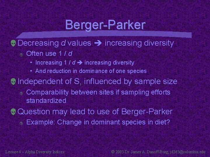
Berger-Parker Decreasing d values increasing diversity þ Often use 1 / d • Increasing 1 / d increasing diversity • And reduction in dominance of one species Independent of S, influenced by sample size þ Comparability between sites if sampling efforts standardized Question may lead to use of Berger-Parker þ Example: Change in dominant species in diet? Lecture 4 – Alpha Diversity Indices © 2003 Dr. James A. Danoff-Burg, jd 363@columbia. edu

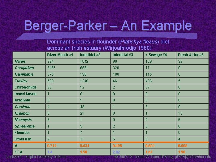
Berger-Parker – An Example Dominant species in flounder (Platichys flesus) diet across an Irish estuary (Wirjoatmodjo 1980) River Mouth #1 Intertidal #2 Intertidal #3 + Sewage #4 Fresh & Hot #5 Nereis 394 1642 90 126 32 Corophium 3487 5681 320 17 0 Gammarus 275 196 180 115 0 Tubifex 683 1348 46 436 5 Chironomids 22 12 2 27 0 Insect larvae 1 0 0 Arachnid 0 1 0 0 0 Carcinus 4 48 1 3 0 Cragnon 6 21 0 1 13 Neomysis 8 1 0 0 9 Sphaeroma 1 5 2 0 0 Flounder 1 7 1 1 0 Other fish 2 3 5 0 4 d 0. 714 0. 634 0. 495 0. 601 0. 508 1/d 1. 4 1. 58 2. 02 1. 67 1. 96 Lecture 4 – Alpha Diversity Indices © 2003 Dr. James A. Danoff-Burg, jd 363@columbia. edu

Berger-Parker Calculations – Worked Example 11 Calculate N, S, Nmax Calculate d and 1/d Very simple Lecture 4 – Alpha Diversity Indices © 2003 Dr. James A. Danoff-Burg, jd 363@columbia. edu

Alpha Diversity Indices Q-Statistic Intro to Alpha Diversity Indices Simpson Mc. Intosh Berger-Parker Shannon-Wiener Brillouin Jack-Knifing Diversity Indices Pielou’s Hierarchical Diversity Index Lecture 4 – Alpha Diversity Indices Week 1 Week 2 © 2003 Dr. James A. Danoff-Burg, jd 363@columbia. edu

Alpha Diversity Indices “Heterogeneity Indices” þ þ Consider both evenness AND richness Species abundance models only consider evenness No assumptions made about species abundance distributions þ þ Cause of distribution Shape of curve “Non-parametric” þ Free of assumptions of normality Lecture 4 – Alpha Diversity Indices © 2003 Dr. James A. Danoff-Burg, jd 363@columbia. edu

Two General Categories Information Theory (complicated computation) þ þ Diversity (or information) of a natural system is similar to info in a code or message Examples: Shannon-Wiener and Brillouin Indices Species Dominance Measures (simple comput. ) þ þ þ Weighted towards abundance of the commonest species Total species richness is downweighted relative to evenness Examples: Simpson, Mc. Intosh, and Berger-Parker Lecture 4 – Alpha Diversity Indices © 2003 Dr. James A. Danoff-Burg, jd 363@columbia. edu

Information Theory, described (read more here) þ A system contains more information when it has many possible states • E. g. , large numbers of species, or high species richness þ Also contains more information when the probability of encountering each state is high • E. g. , all species are equally abundant or have high evenness Indices derived from this simple relationship between richness and evenness þ Examples • Shannon-Wiener and Brillouin Lecture 4 – Alpha Diversity Indices © 2003 Dr. James A. Danoff-Burg, jd 363@columbia. edu

Alpha Diversity Indices Q-Statistic Intro to Alpha Diversity Indices Simpson Mc. Intosh Berger-Parker Shannon-Wiener Brillouin Jack-Knifing Diversity Indices Pielou’s Hierarchical Diversity Index Lecture 4 – Alpha Diversity Indices Week 1 Week 2 © 2003 Dr. James A. Danoff-Burg, jd 363@columbia. edu

Shannon-Wiener Index Derived by Claude Shannon and Warren Weaver in late 40 s þ þ Developed a general model of communication and information theory Initially developed to separate noise from information carrying signals Subsequently þ mathematician Norbert Wiener contributed to the model as part of his work in developing cybernetic technology Called alternatively Shannon-Weaver, Shannon. Wiener, or Shannon Index – more info here Lecture 4 – Alpha Diversity Indices © 2003 Dr. James A. Danoff-Burg, jd 363@columbia. edu

Shannon-Wiener Assumptions þ þ þ All individuals are randomly sampled Population is indefinitely large, or effectively infinite All species in the community are represented Result: difficult to justify for many communities þ þ Particularly very diverse communities, guilds, functional groups Incomplete sampling significant error & bias • Increasingly important as proportion of species sampled declines • Simple mathematical consequence – see next slide Lecture 4 – Alpha Diversity Indices © 2003 Dr. James A. Danoff-Burg, jd 363@columbia. edu

Shannon-Wiener Mathematics Equation þ H’ = -S pi ln pi • pi = proportion of individuals found in the ith species • Unknowable, estimated using ni / N – Flawed estimation, need more sophisticated equation (2. 18 in Magurran) þ Error • Mostly from inadequate sampling • Flawed estimate of pi is negligible in most instances from this simple estimate Lecture 4 – Alpha Diversity Indices © 2003 Dr. James A. Danoff-Burg, jd 363@columbia. edu

Shannon-Wiener Mathematics Need to convert data þ þ Log 2 was historically used Any Log base is acceptable • Need consistency across samples þ Currently, Ln is used more commonly • What we will use Range of S-W index þ þ þ Usually between 1. 5 and 3. 5 Rarely surpasses 4. 5 If underlying distribution is log-normal • Need 100, 000 species to have a H’ > 5. 0 Lecture 4 – Alpha Diversity Indices © 2003 Dr. James A. Danoff-Burg, jd 363@columbia. edu

Building on H’ Can also use Exp H’ þ = Number of equally common species required to produce a given H’ value • Reduces S from the observed value • Allows for an estimation of departures from maximal evenness and diversity þ We won’t explore this here Lecture 4 – Alpha Diversity Indices © 2003 Dr. James A. Danoff-Burg, jd 363@columbia. edu

Building on H’ Evenness measure (E) þ Useful for determining the departure from maximal evenness and diversity • Similar to the Exp H’ þ þ þ Hmax = maximal diversity which could occur if all species collected were equally abundant E = H’ / Hmax = H’ / ln S 0<E<1 • H’ will always be less than Hmax þ þ Assumes all species have been sampled Some have criticized this as being biologically unrealistic • Argue for best fit to the Broken Stick model Lecture 4 – Alpha Diversity Indices © 2003 Dr. James A. Danoff-Burg, jd 363@columbia. edu

Comparing H’ Values Using Shannon for a t-test þ þ Can use a simple t-test for differences between two samples Need variance in H’ (Var H’) and to know the df • Both have complicated equations (2. 19, 2. 21 in Magurran) Shannon and ANOVA þ þ H’ values tend to be normally distributed Can use ANOVAs for differences between multiple sites • Need to have real replication to do this • Pseudoreplication introduces error, particularly in parametric statistics Lecture 4 – Alpha Diversity Indices © 2003 Dr. James A. Danoff-Burg, jd 363@columbia. edu

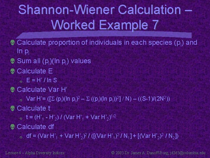
Shannon-Wiener Calculation – Worked Example 7 Calculate proportion of individuals in each species (pi) and ln pi Sum all (pi)(ln pi) values Calculate E þ E = H’ / ln S Calculate Var H’ þ Var H’= ([S (pi)(ln pi)2 – S ((pi)(ln pi))2] / N) – ((S-1)/(2 N 2)) Calculate t þ t = (H’ 1 - H’ 2) / (Var H’ 1 + Var H’ 2)1/2 Calculate df þ df = (Var H’ 1 + Var H’ 2)2 / ([(Var H’ 1)2 / N 1] + [(Var H’ 2)2 / N 2]) Lecture 4 – Alpha Diversity Indices © 2003 Dr. James A. Danoff-Burg, jd 363@columbia. edu

Alpha Diversity Indices Q-Statistic Intro to Alpha Diversity Indices Simpson Mc. Intosh Berger-Parker Shannon-Wiener Brillouin Jack-Knifing Diversity Indices Pielou’s Hierarchical Diversity Index Lecture 4 – Alpha Diversity Indices Week 1 Week 2 © 2003 Dr. James A. Danoff-Burg, jd 363@columbia. edu

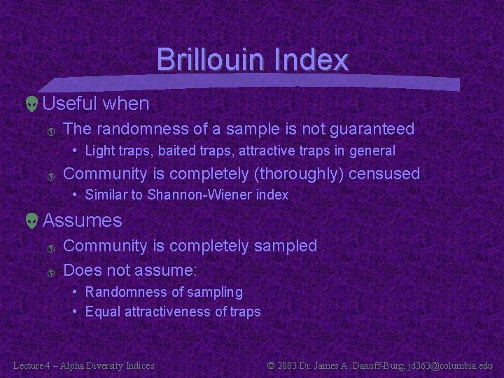
Brillouin Index Useful when þ The randomness of a sample is not guaranteed • Light traps, baited traps, attractive traps in general þ Community is completely (thoroughly) censused • Similar to Shannon-Wiener index Assumes þ þ Community is completely sampled Does not assume: • Randomness of sampling • Equal attractiveness of traps Lecture 4 – Alpha Diversity Indices © 2003 Dr. James A. Danoff-Burg, jd 363@columbia. edu

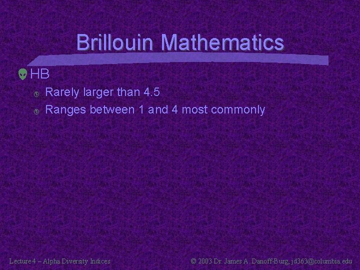
Brillouin Mathematics HB þ þ Rarely larger than 4. 5 Ranges between 1 and 4 most commonly Lecture 4 – Alpha Diversity Indices © 2003 Dr. James A. Danoff-Burg, jd 363@columbia. edu

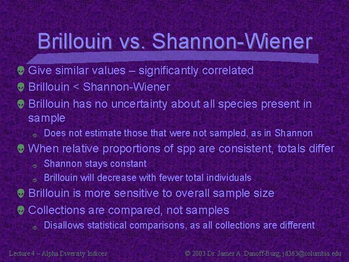
Brillouin vs. Shannon-Wiener Give similar values – significantly correlated Brillouin < Shannon-Wiener Brillouin has no uncertainty about all species present in sample þ Does not estimate those that were not sampled, as in Shannon When relative proportions of spp are consistent, totals differ þ þ Shannon stays constant Brillouin will decrease with fewer total individuals Brillouin is more sensitive to overall sample size Collections are compared, not samples þ Disallows statistical comparisons, as all collections are different Lecture 4 – Alpha Diversity Indices © 2003 Dr. James A. Danoff-Burg, jd 363@columbia. edu

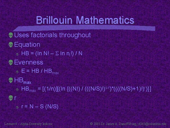
Brillouin Mathematics Uses factorials throughout Equation þ HB = (ln N! – S ln ni!) / N Evenness þ E = HB / HBmax þ HBmax = [(1/n)][(ln {((N!) / (((N/S)!)s-r)*((((N/S)+1)!)r)}] r þ r = N – S (N/S) Lecture 4 – Alpha Diversity Indices © 2003 Dr. James A. Danoff-Burg, jd 363@columbia. edu

Brillouin Calculations – Worked Example 8 Calculate HB Calculate r Calculate HBmax Calculate E Lecture 4 – Alpha Diversity Indices © 2003 Dr. James A. Danoff-Burg, jd 363@columbia. edu

Alpha Diversity Indices Q-Statistic Intro to Alpha Diversity Indices Simpson Mc. Intosh Berger-Parker Shannon-Wiener Brillouin Jack-Knifing Diversity Indices Pielou’s Hierarchical Diversity Index Lecture 4 – Alpha Diversity Indices Week 1 Week 2 © 2003 Dr. James A. Danoff-Burg, jd 363@columbia. edu

Jack-Knifing Diversity Indices Improves the accuracy of any estimate First proposed in 1956 (Quenouille) and refined by Tukey in 1958 þ þ Theoretical biostatisticians First applied to diversity by Zahl in 1977 Lecture 4 – Alpha Diversity Indices © 2003 Dr. James A. Danoff-Burg, jd 363@columbia. edu

Jack-Knifing Assumptions: þ þ None made about underlying distribution Does not attempt to estimate actual number of species present • As in Shannon-Wiener Random sampling is not necessary þ þ Repeated measures overcome the biases Jack-Knifing can determine the impact of biased sampling Lecture 4 – Alpha Diversity Indices © 2003 Dr. James A. Danoff-Burg, jd 363@columbia. edu

Data for Jack-Knifing Need multiple samples to conduct this procedure þ Some debate exists about this, may be able to do a single sample For our data þ þ Can use each tray to create an estimate for what? Can use each garden to create an estimate for what? Lecture 4 – Alpha Diversity Indices © 2003 Dr. James A. Danoff-Burg, jd 363@columbia. edu

Jack-Knifing Procedure þ þ þ Create the overall pooled index estimate ( Subsamples with replacement from the actual data Creates pseudovalues of the statistic Pseudovalues are normally distributed about the mean Mean value is best estimate of the statistics Confidence limits þ þ Also possible to attach these to the estimate Consequence of normal distribution of pseudovalues Lecture 4 – Alpha Diversity Indices © 2003 Dr. James A. Danoff-Burg, jd 363@columbia. edu

Applications of the Jack-Knife Most commonly used for the most common indices þ þ Shannon and Simpson in particular Also useful for other indices Variance in the pseudovalues þ þ More useful than the Var H’ of the Shannon Gives a better estimate of the accuracy and impact of non-random sampling Lecture 4 – Alpha Diversity Indices © 2003 Dr. James A. Danoff-Burg, jd 363@columbia. edu

Jack-Knifing – Worked Example 12 Overall diversity index including all data (V) Recalculate, excluding each sample in turn þ Creates n number of VJi estimates Convert VJi to pseudovalues VPi þ þ Use VPi = (n. V) – [(n-1) (VJi)] n = number of samples Calculate mean VP value Calculate Sample Influence Function þ SIF = V – VP Calculate standard error VP = stand dev Vpis / n Lecture 4 – Alpha Diversity Indices © 2003 Dr. James A. Danoff-Burg, jd 363@columbia. edu

Alpha Diversity Indices Q-Statistic Intro to Alpha Diversity Indices Simpson Mc. Intosh Berger-Parker Shannon-Wiener Brillouin Jack-Knifing Diversity Indices Pielou’s Hierarchical Diversity Index Lecture 4 – Alpha Diversity Indices Week 1 Week 2 © 2003 Dr. James A. Danoff-Burg, jd 363@columbia. edu

Pielou’s Pooled Quadrat Method Similar to Jack-Knifing þ Improves the estimate of diversity Also not influenced by non-random sampling þ Provides the best estimate of the value, given the data Can be calculated using either of the information statistic indexes þ þ Shannon Brillouin Lecture 4 – Alpha Diversity Indices © 2003 Dr. James A. Danoff-Burg, jd 363@columbia. edu

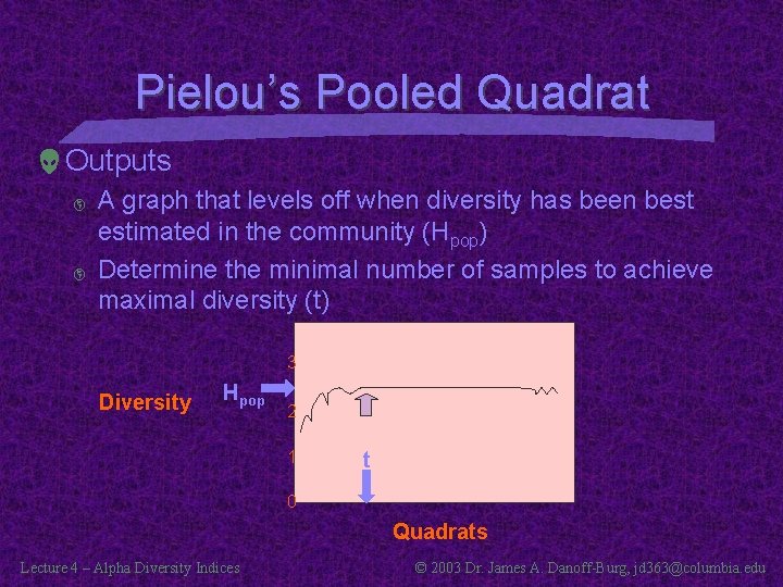
Pielou’s Pooled Quadrat Outputs þ þ A graph that levels off when diversity has been best estimated in the community (Hpop) Determine the minimal number of samples to achieve maximal diversity (t) 3 Diversity Hpop 2 1 t 0 Quadrats Lecture 4 – Alpha Diversity Indices © 2003 Dr. James A. Danoff-Burg, jd 363@columbia. edu

Pielou’s Method Utility Stability of an index þ Evaluating the stability of a diversity index and its relationship to sample size Determining an adequate sample size þ þ Produces a graph of the indices When the line levels out, you have adequate samples • Adequately estimated biodiversity locally Can create confidence limits þ þ Then, can compare values between habitats Use standard parametric statistics Lecture 4 – Alpha Diversity Indices © 2003 Dr. James A. Danoff-Burg, jd 363@columbia. edu

Pielou’s Pooled Quadrat – Worked Example 13 Using Brillouin index, calculate all HBk þ þ From k = 0 k = z k = number of samples z = total samples Mk = total abundance in k number of samples Estimate t þ t = Point at which HBk levels off Calculate Hpop þ þ þ Using k+t number of samples Calculate mean Hpop Calculate standard deviation Lecture 4 – Alpha Diversity Indices © 2003 Dr. James A. Danoff-Burg, jd 363@columbia. edu

Next week(s): Continuing Alpha Diversity Indices Read þ þ Magurran Ch 2, pages 32 -45 Magurran Worked Examples 6 -13 We will continue conducting alpha diversity analyses next week Lecture 4 – Alpha Diversity Indices © 2003 Dr. James A. Danoff-Burg, jd 363@columbia. edu

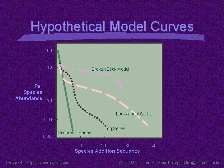
Hypothetical Model Curves 100 10 Broken Stick Model Per 1 Species Abundance 0. 1 Log-Normal Series 0. 01 0. 001 Geometric Series 10 Log Series 20 30 40 Species Addition Sequence Lecture 4 – Alpha Diversity Indices © 2003 Dr. James A. Danoff-Burg, jd 363@columbia. edu