Alignment scoring statistics and scoring matrices Analysis of

Alignment scoring statistics and scoring matrices Analysis of Biological Sequences

Two sequences Which is the better alignment? How can we tell? We need a scoring function. For example, match = 2, mismatch = -1, gap = -2. Then aln #1 scores 0 and aln #2 scores 6.

Different scoring rules -> different alignments Dynamic programming: global alignment Match=5, mismatch = -4, gap w = -7

Different scoring rules -> different alignments Dynamic programming: global alignment Match=5, mismatch = -4, gap w = -2

Scoring rules/matrices • Why are they important? – Choice of scoring rule can dramatically influence the sequence alignments obtained and, therefore, the analysis being done – Different scoring matrices have been developed for different situations; using the wrong one can make a big difference. • What do they mean? – Scoring matrices implicitly represent a particular theory of evolution – Elements of the matrices specify relationships between amino acid residues or nucleotides

Substitution Matrices We need scoring terms for each aligned residue pair • Models: Random model (R): letter a occurs with frequency qa Sequence x: Sequence y:

Substitution matrices Log-odds ratio -> log likelihood ratio that the pair (a, b) is related vs unrelated (depends on scoring matrices) The alignment score is the log likelihood that the sequences have common ancestry

Two major scoring matrices • PAM = accepted point mutation – 71 trees with 1572 accepted mutations, sequences with >85% identity – PAM 1 means average of 1% change over all amino acids – 1 PAM = 10 my evolutionary distance • BLOSUM = Blocks substitution matrices – Based on BLOCKS database (Henikoff & Henikoff, 1992) of over 2000 conserved amino acid patterns in over 500 proteins

PAM matrices • Amino acid changes are modeled by a Markov process, so each mutation is independent of previous mutations – This means that we can calculate the matrices for more distantly related proteins by multiplying matrices for closely related proteins (PAM 250 = PAM 1 multiplied by itself 250 times) – PAM 250 = 250% change over 2500 my. – ~20% similarity at this level; shown to be best for proteins of 14 -27% similarity

PAM matrices • PAM 120: 40% similarity • PAM 80: 50% similarity • PAM 60: 60% similarity • Simulations have confirmed these numbers • Choosing the best PAM matrix: ungapped alignment score will be highest when the correct matrix is used.

PAM matrices—assumptions • • • ~ P(X->Y) = P(Y->X) P(X->Z->Y) is low in a single PAM period Markov model/independence Each change in current AA at a particular site is independent of previous mutational event • All sequences have similar amino acid composition • Change is independent of position of AA

PAM Construction • Organize related sequence by phylogenetic tree • The number of changes of each amino acid into every other amino acid is counted (We also need to know the relative amount of change for each amino acid. • Relative mutability is calculated by changes of each amino acid divided by exposure to mutation

Relative Mutability • In each group of related sequence, the number of changes of each amino acid / Exposure to mutation • Exposure of mutation= Frequency of occurrence of the amino acid in the group of sequences being analyzed X Total number of all amino acid changes that occurred in that group per 100 sites

Calculation of relative mutability of amino acid • Find frequency of amino acid change at a certain position in protein. • Divide the frequency by the frequency that the amino acid occurs in all proteins. This gives the mutabilities of all amino acids. • Multiply the alanine mutability by a factor to get the value 100. • Multiply the 19 other a. a. mutabilities by the same factor. • Result: Relative Mutabilities

Relative Mutabilities of amino acids Asn Ser Asp Glu Ala Thr Ile Met Gln Val 134 120 106 102 100 97 96 94 93 74 His Arg Lys Pro Gly Tyr Phe Leu Cys Trp 66 65 56 56 49 41 41 40 20 18

Why are the mutabilities different? • High mutabilities because a similar amino acid can replace it. (Asp for Glu) • Conversely, the low mutabilities are unique, can’t be replaced.

An example: obtaining the PAM 250 score for Tyr <->Phe (from Mount book) • Original PAM data: 1572 observed amino acid changes, 260 were between Phe and Tyr • 260/1572 is multiplied by relative mutability of Phe and by the pair exchange frequency->mutation probability score • Relative mutability = chance that the amino acid will change (Dayhoff used # times observed to change) • Pair exchange frequency = fraction of Phe->Tyr/all Phe mutations • Normalize to a sum of 1% probability of any amino acid change, then take log odds -> PAM 1

Example: Tyr<->Phe 260/1572 x mutability x pair exchange frequency THEN normalize to 1% change over whole matrix Normalized probability scores for some Phe mutations aa change F->A F->R F->F F->Y PAM 1 0. 0002 0. 0001 0. 9946 0. 0021 PAM 250 0. 04 0. 01 0. 32 0. 15

Example: Tyr/Phe • PAM 1 multiplied by itself 250 times, now Phe->Tyr is 0. 15 and Tyr->Phe is 0. 20 Log odds: log(prob. score/frequency in sequence) Phe->Tyr: log(0. 15/0. 040) = 0. 57 Tyr->Phe: log(0. 20/0. 03) = 0. 83 Multiply log odds by 10, take the average, and this is the PAM 250 log odds score for F<->Y ((5. 7+8. 3)/2 = 7) 7>0 -> favorable mutation

BLOSUM • Henikoff & Henikoff used PROTOMAT program to create BLOCKS database from Prosite catalog • PROTOMAT looks for A 1 -d 1 -A 2 -d 2 -A 3 where A 1, A 2, A 3 are conserved residues and d 1, d 2 < 25 residue intervening sequence • These initial patterns are consolidated into larger patterns by PROTOMAT • Sequences above a similarity threshold are clustered into families (% threshold -> BLOSUM #)

BLOSUM construction 1. Count mutations

BLOSUM construction 2. Tallying mutation frequencies qij = # times amino acid j mutates to amino acid i Since we don’t know ancestry, each mutation gets entered twice

BLOSUM construction 3. Matrix of mutation probabilities • Create probabilities from mutation frequencies

BLOSUM construction 4. Calculate abundance of each residue (Marginal probability) pi is the marginal probability, meaning the expected probability of occurrence of amino acid i

BLOSUM construction 5. Obtaining a BLOSUM matrix • BLOSUM is a log-likelihood matrix: Sij = 2 log 2(pij/(pipj))

Building BLOSUM Matrices (cont. ) Which BLOSUM to use? BLOSUM 80 62 35 Identity 80% 62% (usually default value) 35% If you are comparing sequences that are very similar, use BLOSUM 80. Sequence comparisons that are more divergent (dissimilar) than 20% are given very low scores in this matrix.

Choice of scoring matrix BLOSUM 100 PAM 250 PAM 1 BLOSUM 30 Similarity Ev. distance Seq. length

BLOSUM vs PAM • BLOSUM: based on short conserved sequences (blocks) – – – Based on a range of evolutionary periods Each matrix constructed separately Indirectly accounts for interdependence of residues Range of sequences, range of replacements Overcounts related mutations Designed to find their conserved domain • PAM: evolutionary model – – – Based on extrapolation from a short evolutionary period Errors in PAM 1 are magnified through PAM 250 Assumes Markov process Many sequences depart from average composition Rare replacements too infrequent to be represented accurately Designed to track the evolutionary origin

Issues • Both BLOSUM and PAM matrices are derived from small sets of sequences from biased databases • Both types of matrices require aligned sequences for their construction • Both types of matrices depend on global, ungapped alignments

Which Scoring Matrix to use? PAM-1 BLOSUM-100 PAM-250 BLOSUM-20 • Small evolutionary distance • High identity within short sequences • Large evolutionary distance • Low identity within long sequences

Other matrix types • Simple identity • Scored according to codon tables and also with added information based on structural similarity of aa side chain • Chemical properties of amino acids • 3 D structural alignments • Dipeptide-based • Family-specific (kinase, transmembrane etc) • DNA

Determining correct alignment • Can also use information theory/relative entropy to score alignments

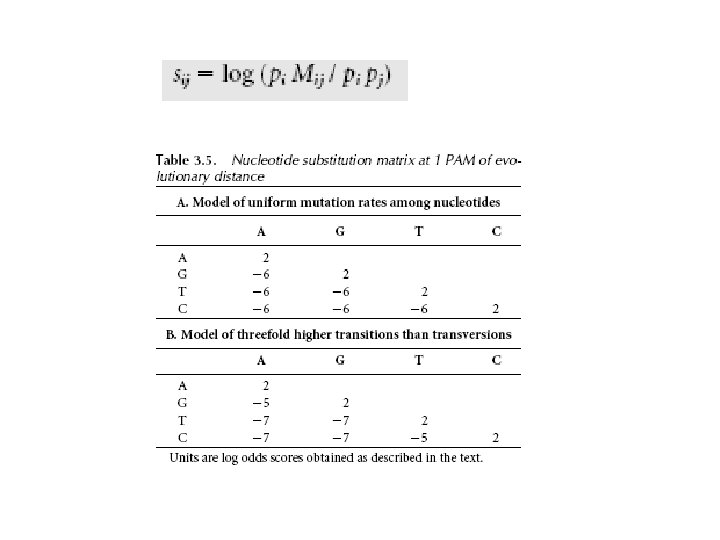
Nucleic Acid PAM Scoring scheme • PAM 1 mutation matrix representing 99% conservation and 1% mutation was calculated • The matrix value is used to produce log odd scoring matrix (Frequency of substitution expected at increasing evolutionary distances)

Gap penalties • Until now we have talked about ungapped alignments and their properties • Inclusion of gaps and gap penalties is necessary to obtain the best alignment g = opening penalty wx = g + rx r = penalty for extending gap or w = gap penalty (for opening gap) wx = g + r(x-1) x = length of the gap This is the affine gap penalty.

Penalties of Gaps at the ends of alignments • If comparing sequences that are homologous and of about same length, it makes a great deal of senses to include end gap penalties to achieve best overall alignment. • Otherwise do not use end gap penalties.

Assessing the significance of sequence alignments • Local alignments are rarely produced between random sequences • Global alignments are readily produced between random sequences -> harder to assess the significance of a global alignment • Can approximate a score by shuffling the sequences and realigning but this can be misleading • Alignment scores follow the extreme value Gumbel distribution, not a normal distribution

Assessing the significance of sequence alignments Alignment scores