Algoritmi rasterske grafike Risanje primitivov Vector displays paint

- Slides: 132

Algoritmi rasterske grafike

Risanje primitivov • Vector displays “paint” lines across the smooth phosphor coating of the screen and generate smooth curves or straight lines. • Raster-scan based displays work on a grid principle and are inherently unable to represent smooth curves. • Mass-market computer displays are based on the raster-scan method.

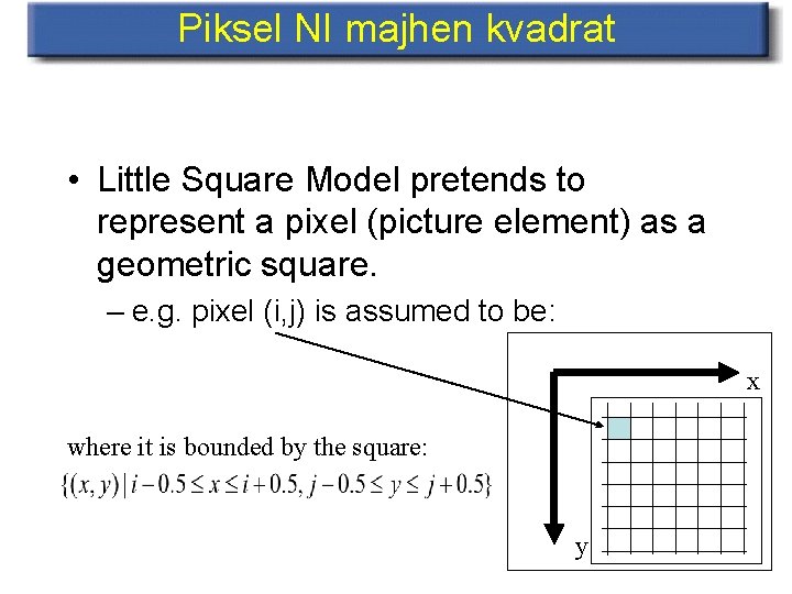
Piksel NI majhen kvadrat • Little Square Model pretends to represent a pixel (picture element) as a geometric square. – e. g. pixel (i, j) is assumed to be: x where it is bounded by the square: y

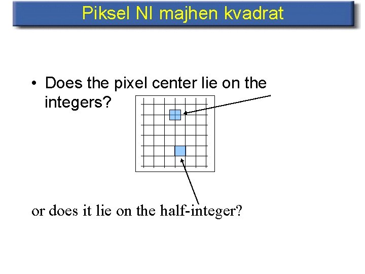
Piksel NI majhen kvadrat • Does the pixel center lie on the integers? or does it lie on the half-integer?

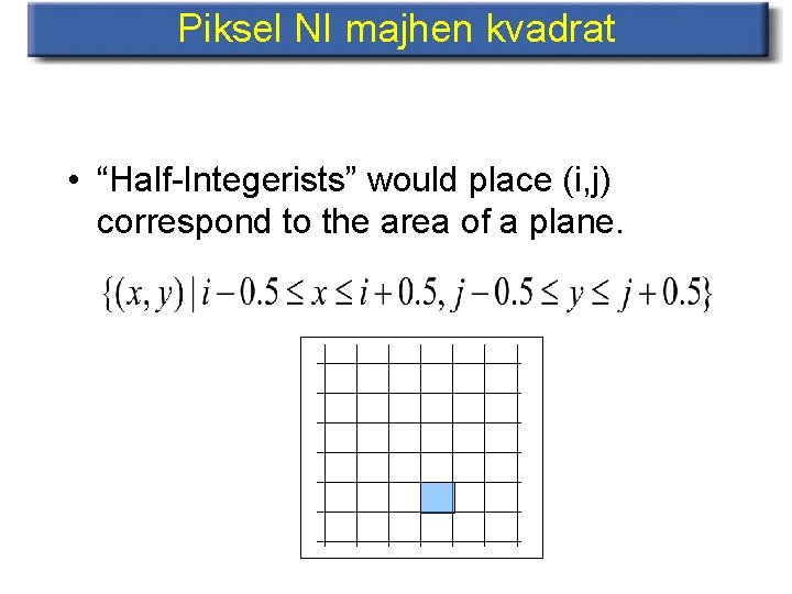
Piksel NI majhen kvadrat • “Half-Integerists” would place (i, j) correspond to the area of a plane.

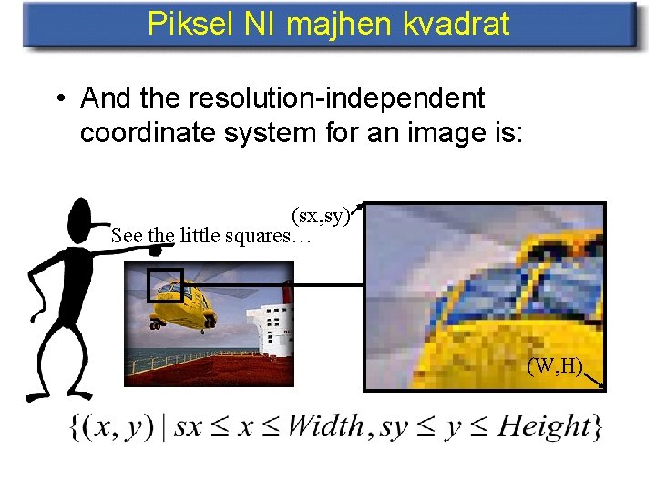
Piksel NI majhen kvadrat • And the resolution-independent coordinate system for an image is: (sx, sy) See the little squares… (W, H)

Piksel NI majhen kvadrat • A pixel is a point sample. • It only exists at a point. • A colour pixel will actually contain 3 samples: red, green and blue • A pixel is not a little square. • An image is a rectilinear array of point samples (discrete not continuous)

Piksel NI majhen kvadrat • Why is the “little square model” popular: – Rendering (conversion of abstract geometry into viewable pixels) – The mathematics is easier if we assume a continuum.

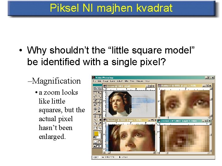
Piksel NI majhen kvadrat • Why shouldn’t the “little square model” be identified with a single pixel? –Magnification • a zoom looks like little squares, but the actual pixel hasn’t been enlarged.

Piksel NI majhen kvadrat • Why shouldn’t the “little square model” be identified with a single pixel? –Scanner Digitising a Picture –a light source illuminates the paper –light reflected is collected and measured by a colour sensitive device –the collected light is passed through a filtering shape (never a square) –pixels are determined by averaging overlapping shapes.

Uvod v 2 D upodabljanje • 2 D primitives – – Line segments Ellipses and circles Polygons Curves • Rasterization (Scan-Conversion) – Turn 2 D primitives into sets of pixels – A Pixel Is Not A Little Square (Digital Signal Processing) – Antialiasing • Clipping – Compute the intersection of a primitive and a shape – Primitive: line segment, polygon – Shape: rectangle, convex polygon

Nekaj matematike • Coordinate system: y axis upward or downward? • Pixels are at the centres of integer coordinates • Line segments – – Equation of a (2 D) line: ax + by + c = 0 Direction: (-b a) Normal vector: (a b) Parametric equation of a segment [P 1 -P 2] x(t) = x 1 + t*(x 2 -x 1) = (1 -t)*x 1 + t*x 2 y(t) = y 1 + t*(y 2 -y 1) = (1 -t)*y 1 + t*y 2 t in [0. . 1]

Nekaj matematike • Polygons – Closed sequence of line segments (P 1 P 2. . Pn) – Different types – Convex – Concave = not convex – Self-intersecting (8 -shape) – With holes

Rasterizacija • Converting mathematical definitions to pixels – We can only approximate the mathematical definition • A Pixel is Not a Little Square • Avoid holes • Draw each pixel exactly once – Naive (expensive) approach • Evaluate formulas on the pixel grid – Clever approach • • Use integer calculations Avoid divides and multiplies Use incremental computations Use spatial coherence

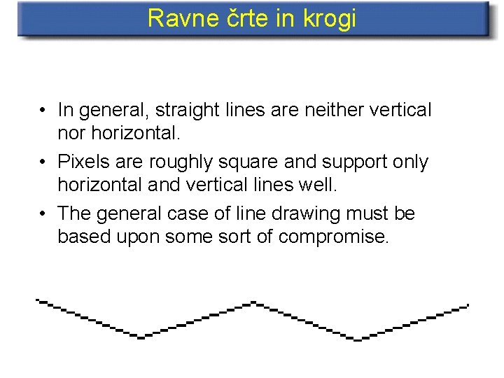
Ravne črte in krogi • In general, straight lines are neither vertical nor horizontal. • Pixels are roughly square and support only horizontal and vertical lines well. • The general case of line drawing must be based upon some sort of compromise.

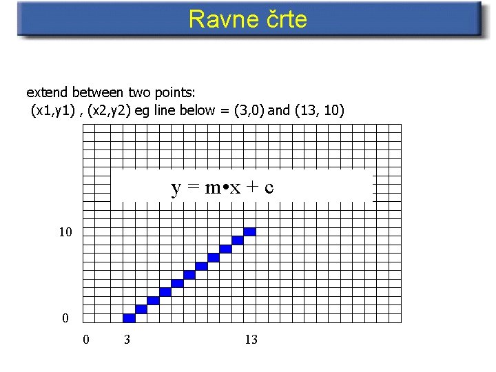
Ravne črte extend between two points: (x 1, y 1) , (x 2, y 2) eg line below = (3, 0) and (13, 10) y = m • x + c 10 0 0 3 13

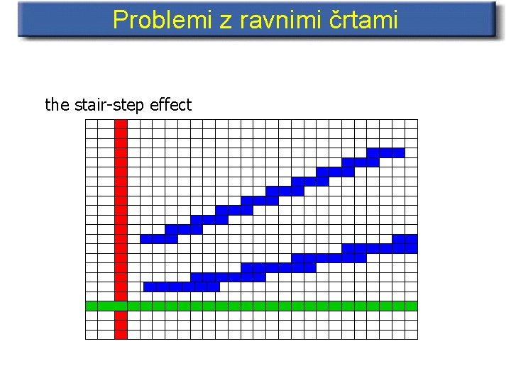
Problemi z ravnimi črtami the stair-step effect

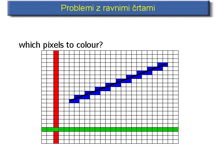
Problemi z ravnimi črtami which pixels to colour?

Približno risanje črt • Assume square pixels. • Assume that the line starts at (x 1, y 1) and finishes at (x 2, y 2). • Say that dx=x 2 -x 1, dy=y 2 -y 1 • If we start with the simplest non-trivial case where dx=dy, we can immediately see that a 45 degree diagonal line has one x step per y step.

Približno risanje črt • The basic requirement for an approximation is to generate the minimum error at each step. • The largest acceptable error must be half a pixel. • To simplify the problem, we consider only one eighth of the possible angles, ie we choose to consider only one octant. We can generalise later using a mirroring technique.

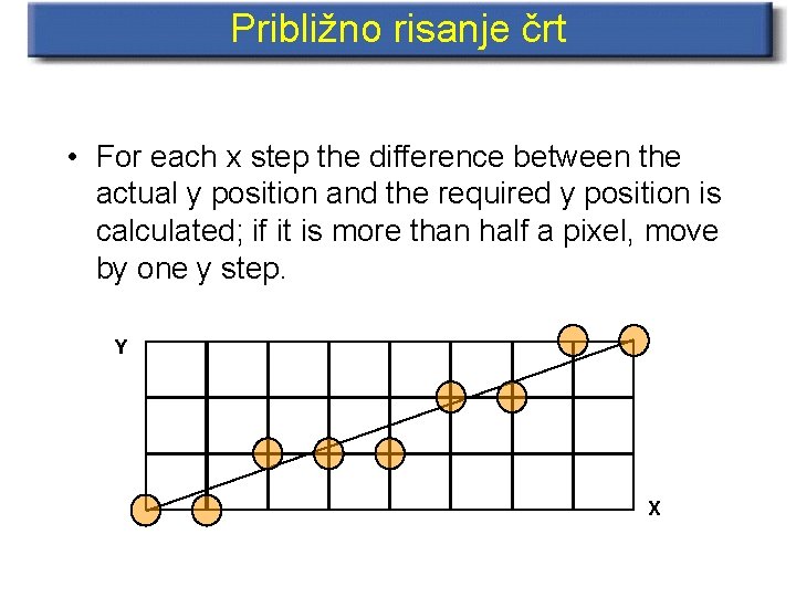
Približno risanje črt • For each x step the difference between the actual y position and the required y position is calculated; if it is more than half a pixel, move by one y step. Y X

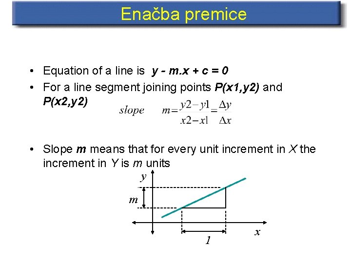
Enačba premice • Equation of a line is y - m. x + c = 0 • For a line segment joining points P(x 1, y 2) and P(x 2, y 2) • Slope m means that for every unit increment in X the increment in Y is m units y m 1 x

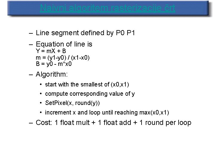
Naivni algoritem rasterizacije črt – Line segment defined by P 0 P 1 – Equation of line is Y = m. X + B m = (y 1 -y 0) / (x 1 -x 0) B = y 0 - m*x 0 – Algorithm: • start with the smallest of (x 0, x 1) • compute corresponding value of y • Set. Pixel(x, round(y)) • increment x and loop until reaching max(x 0, x 1) – Cost: 1 float mult + 1 float add + 1 round per loop

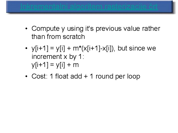
Inkrementalni algoritem rasterizacije črt • Compute y using it's previous value rather than from scratch • y[i+1] = y[i] + m*(x[i+1]-x[i]), but since we increment x by 1: y[i+1] = y[i] + m • Cost: 1 float add + 1 round per loop

Minimiziranje računanj s plavajočo vejico With straight lines one way of minimising the amount of floating point calculation is: if (x 1 = = x 2) => vertical line elseif (y 1 = = y 2) => horizontal line else yk+1 = yk + m Allows the minimum of floating point calculation to be carried out.

Digitalni diferencialni analizator (DDA) • Digital Differential Analyzer algorithm more popularly known as DDA • This is an Incremental algorithm i. e. at each step it makes incremental calculations based on the calculations done during the preceding step • The algorithm uses floating point operations, which are very cleverly avoided in an algorithm first proposed by J. Bresenham of IBM, . The algorithm is well known as Bresenham’s Line Drawing Algorithm. • A slight variation – Midpoint Line Drawing Algorithm –

Bresenham’s Line Algorithm (BLA) • Scan-converts lines using only incremental integer calculations. • BLA again assumes the line is sampled at unit x intervals. • BLA uses the sign (+ve/-ve) of an integer (p) whose value is proportional to: • the difference between the two candidate y values separation from the calculated line path • The differential line algorithm uses floating-point values (the error value is a fraction) and floating point calculations are slow compared with integer calculations. • BLA can be used for curves as well as straight lines. Demo

Digitalni diferencialni analizator (DDA) The DDA is a scan-conversion algorithm, which recognises that the x interval is always 1 (corresponding to moving to the next pixel column in the frame buffer) thus yk+1 = yk + m and the nearest scan-line to yk+1 will be given by: y = (int) (yk+1 + 0. 5)

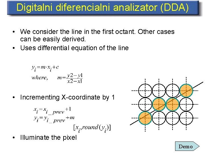
Digitalni diferencialni analizator (DDA) • We consider the line in the first octant. Other cases can be easily derived. • Uses differential equation of the line • Incrementing X-coordinate by 1 • Illuminate the pixel Demo

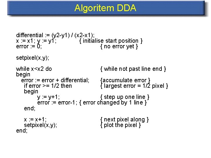
Algoritem DDA differential : = (y 2 -y 1) / (x 2 -x 1); x : = x 1; y : = y 1; { initialise start position } error : = 0; { no error yet } setpixel(x, y); while x<x 2 do { while not past line end } begin error : = error + differential; {accumulate error } if error >= 1/2 then { largest error = 1/2 pixel } begin y : = y+1; { step up one line } error : = error-1; { error changed by 1 line } end; x : = x+1; setpixel(x, y); end; { next pixel along } { plot the pixel }

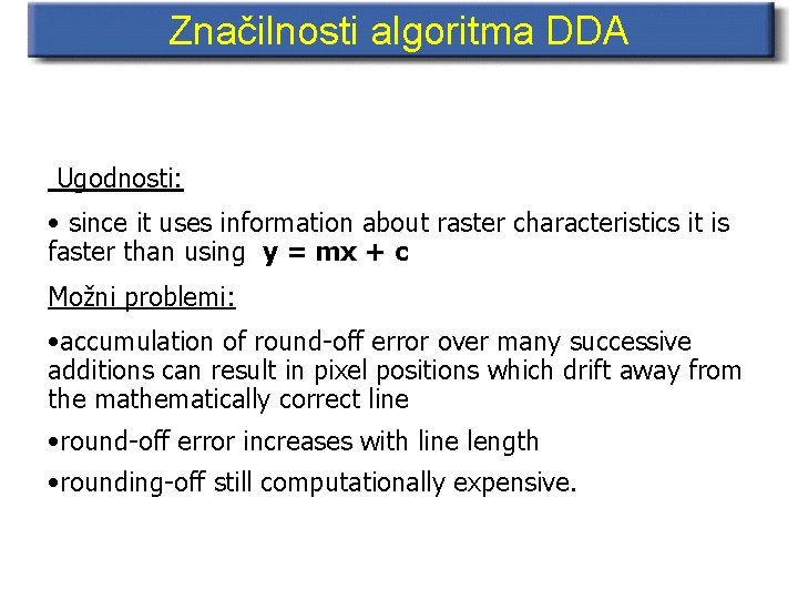
Značilnosti algoritma DDA Ugodnosti: • since it uses information about raster characteristics it is faster than using y = mx + c Možni problemi: • accumulation of round-off error over many successive additions can result in pixel positions which drift away from the mathematically correct line • round-off error increases with line length • rounding-off still computationally expensive.

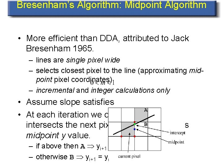
Bresenham’s Algorithm: Midpoint Algorithm • More efficient than DDA, attributed to Jack Bresenham 1965. – lines are single pixel wide – selects closest pixel to the line (approximating midpoint pixel coordinates) – incremental and integer calculations only • Assume slope satisfies • At each iteration we determine if the line intersects the next pixel above or below its midpoint y value. – if above then A yi+1 = yi+1 – otherwise B yi+1 = yi

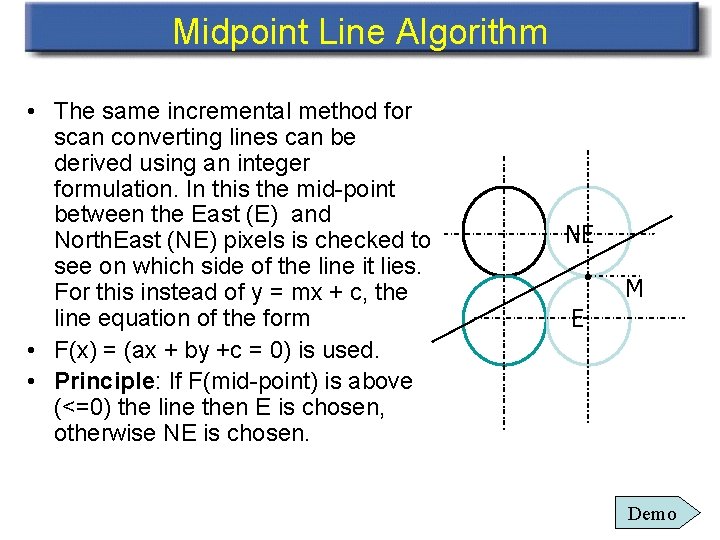
Midpoint Line Algorithm • The same incremental method for scan converting lines can be derived using an integer formulation. In this the mid-point between the East (E) and North. East (NE) pixels is checked to see on which side of the line it lies. For this instead of y = mx + c, the line equation of the form • F(x) = (ax + by +c = 0) is used. • Principle: If F(mid-point) is above (<=0) the line then E is chosen, otherwise NE is chosen. NE • M E Demo

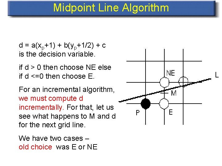
Midpoint Line Algorithm d = a(xp+1) + b(yp+1/2) + c is the decision variable. if d > 0 then choose NE else if d <=0 then choose E. For an incremental algorithm, we must compute d incrementally. For that, let us see what happens to M and d for the next grid line. We have two cases – old choice was E or NE

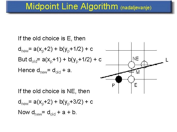
Midpoint Line Algorithm (nadaljevanje) If the old choice is E, then dnew= a(xp+2) + b(yp+1/2) + c But dold= a(xp+1) + b(yp+1/2) + c Hence dnew= dold + a. If the old choice is NE, then dnew= a(xp+2) + b(yp+3/2) + c Now dnew= dold + a + b.

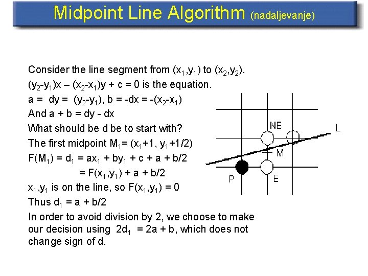
Midpoint Line Algorithm (nadaljevanje) Consider the line segment from (x 1, y 1) to (x 2, y 2). (y 2 -y 1)x – (x 2 -x 1)y + c = 0 is the equation. a = dy = (y 2 -y 1), b = -dx = -(x 2 -x 1) And a + b = dy - dx What should be to start with? The first midpoint M 1= (x 1+1, y 1+1/2) F(M 1) = d 1 = ax 1 + by 1 + c + a + b/2 = F(x 1, y 1) + a + b/2 x 1, y 1 is on the line, so F(x 1, y 1) = 0 Thus d 1 = a + b/2 In order to avoid division by 2, we choose to make our decision using 2 d 1 = 2 a + b, which does not change sign of d.

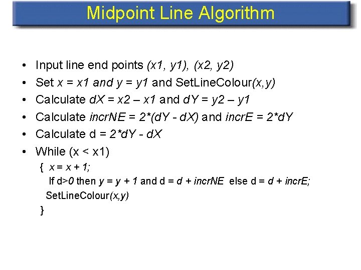
Midpoint Line Algorithm • • • Input line end points (x 1, y 1), (x 2, y 2) Set x = x 1 and y = y 1 and Set. Line. Colour(x, y) Calculate d. X = x 2 – x 1 and d. Y = y 2 – y 1 Calculate incr. NE = 2*(d. Y - d. X) and incr. E = 2*d. Y Calculate d = 2*d. Y - d. X While (x < x 1) { x = x + 1; If d>0 then y = y + 1 and d = d + incr. NE else d = d + incr. E; Set. Line. Colour(x, y) }

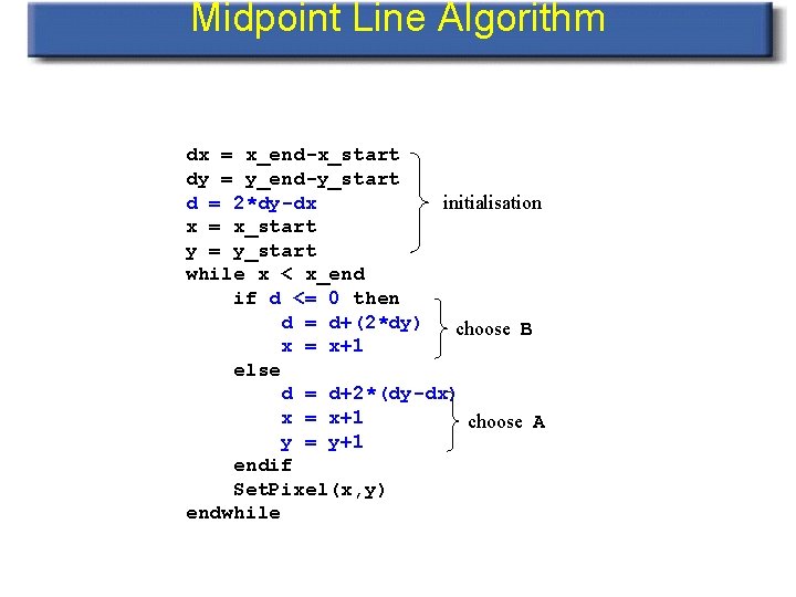
Midpoint Line Algorithm dx = x_end-x_start dy = y_end-y_start d = 2*dy-dx initialisation x = x_start y = y_start while x < x_end if d <= 0 then d = d+(2*dy) choose B x = x+1 else d = d+2*(dy-dx) x = x+1 choose A y = y+1 endif Set. Pixel(x, y) endwhile

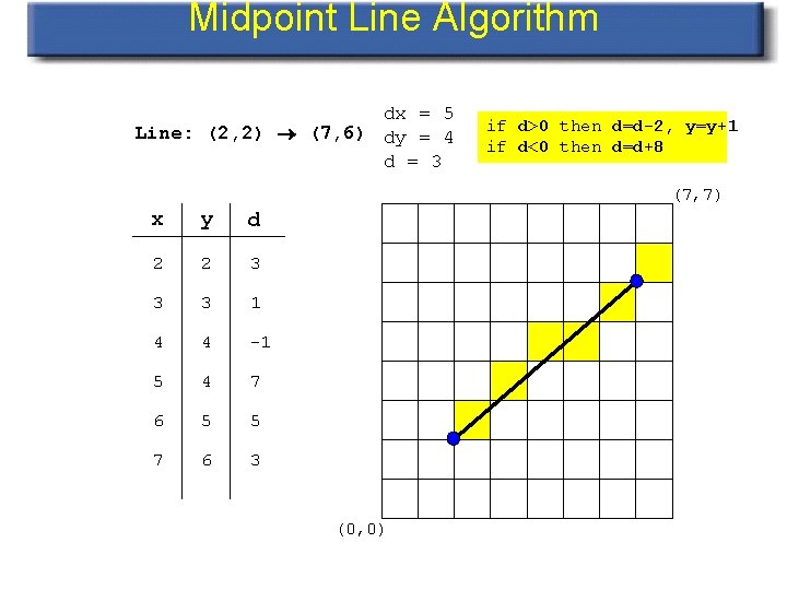
Midpoint Line Algorithm dx = 5 Line: (2, 2) (7, 6) dy = 4 d = 3 if d>0 then d=d-2, y=y+1 if d<0 then d=d+8 (7, 7) x y d 2 2 3 3 3 1 4 4 -1 5 4 7 6 5 5 7 6 3 (0, 0)

Advantages of Incremental Midpoint Line Algorithm • It is an incremental algorithm • It uses only integer arithmetic • Provides the best fit approximation to the actual line

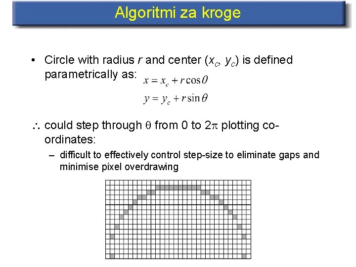
Algoritmi za kroge • Circle with radius r and center (xc, yc) is defined parametrically as: could step through q from 0 to 2 p plotting coordinates: – difficult to effectively control step-size to eliminate gaps and minimise pixel overdrawing

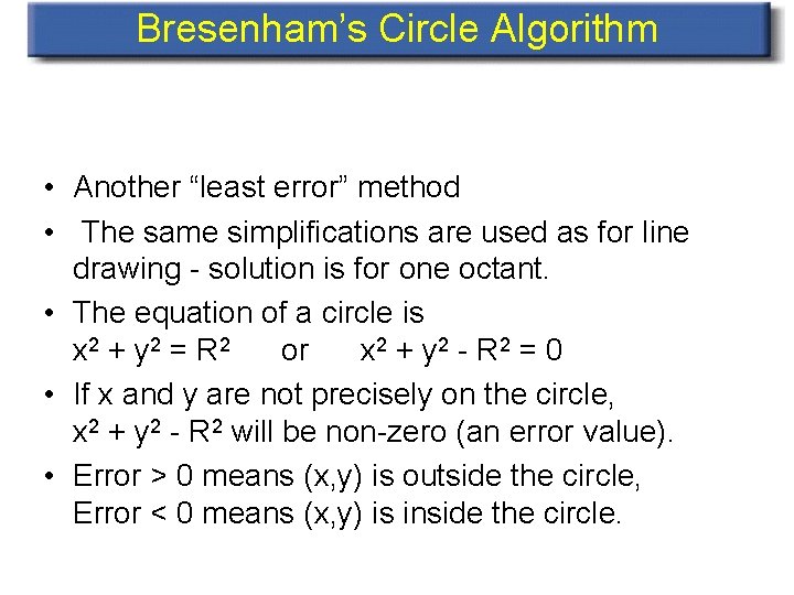
Bresenham’s Circle Algorithm • Another “least error” method • The same simplifications are used as for line drawing - solution is for one octant. • The equation of a circle is x 2 + y 2 = R 2 or x 2 + y 2 - R 2 = 0 • If x and y are not precisely on the circle, x 2 + y 2 - R 2 will be non-zero (an error value). • Error > 0 means (x, y) is outside the circle, Error < 0 means (x, y) is inside the circle.

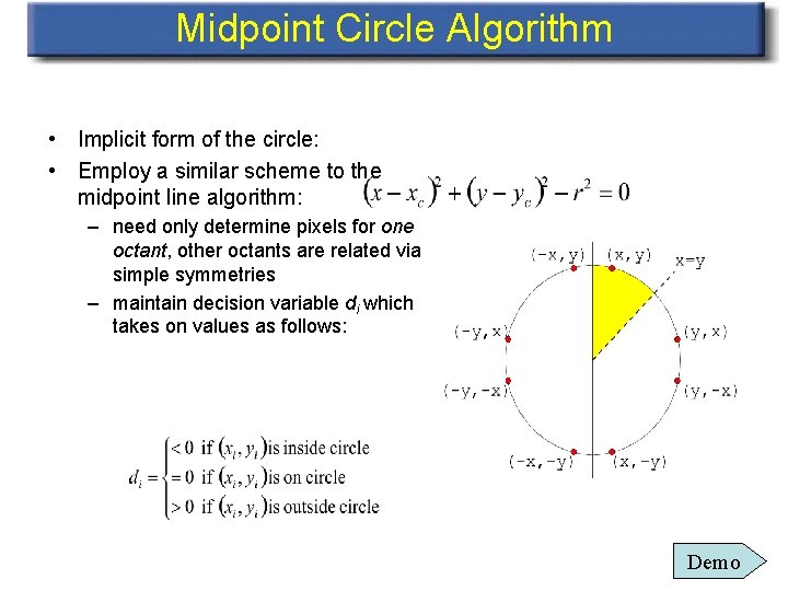
Midpoint Circle Algorithm • Implicit form of the circle: • Employ a similar scheme to the midpoint line algorithm: – need only determine pixels for one octant, other octants are related via simple symmetries – maintain decision variable di which takes on values as follows: Demo

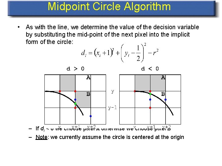
Midpoint Circle Algorithm • As with the line, we determine the value of the decision variable by substituting the mid-point of the next pixel into the implicit form of the circle: – If di < 0 we choose pixel A otherwise we choose pixel B – Note: we currently assume the circle is centered at the origin

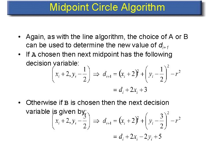
Midpoint Circle Algorithm • Again, as with the line algorithm, the choice of A or B can be used to determine the new value of di+1 • If A chosen then next midpoint has the following decision variable: • Otherwise if B is chosen the next decision variable is given by:

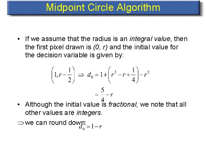
Midpoint Circle Algorithm • If we assume that the radius is an integral value, then the first pixel drawn is (0, r) and the initial value for the decision variable is given by: • Although the initial value is fractional, we note that all other values are integers. we can round down:

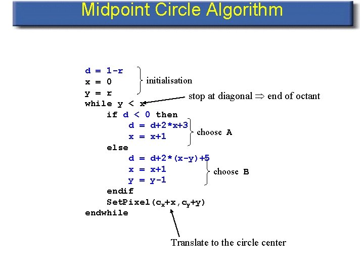
Midpoint Circle Algorithm d = 1 -r initialisation x = 0 y = r stop at diagonal end of octant while y < x if d < 0 then d = d+2*x+3 choose A x = x+1 else d = d+2*(x-y)+5 x = x+1 choose B y = y-1 endif Set. Pixel(cx+x, cy+y) endwhile Translate to the circle center

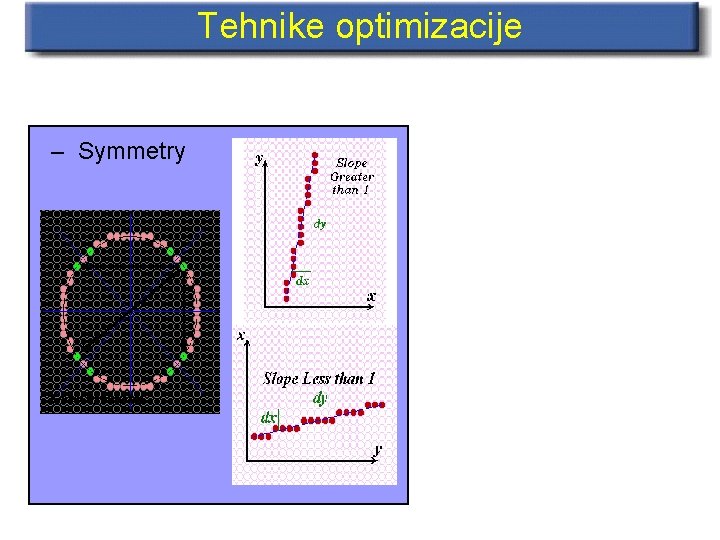
Tehnike optimizacije – Symmetry

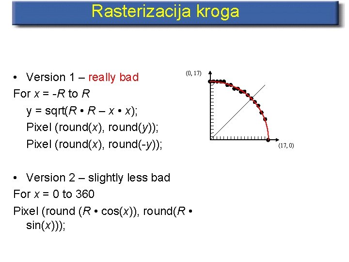
Rasterizacija kroga • Version 1 – really bad For x = -R to R y = sqrt(R • R – x • x); Pixel (round(x), round(y)); Pixel (round(x), round(-y)); (0, 17) • Version 2 – slightly less bad For x = 0 to 360 Pixel (round (R • cos(x)), round(R • sin(x))); (17, 0)

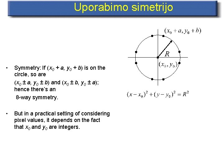
Uporabimo simetrijo R • Symmetry: If (x 0 + a, y 0 + b) is on the circle, so are (x 0 ± a, y 0 ± b) and (x 0 ± b, y 0 ± a); hence there’s an 8 -way symmetry. • But in a practical setting of considering pixel values, it depends on the fact that x 0 and y 0 are integers.

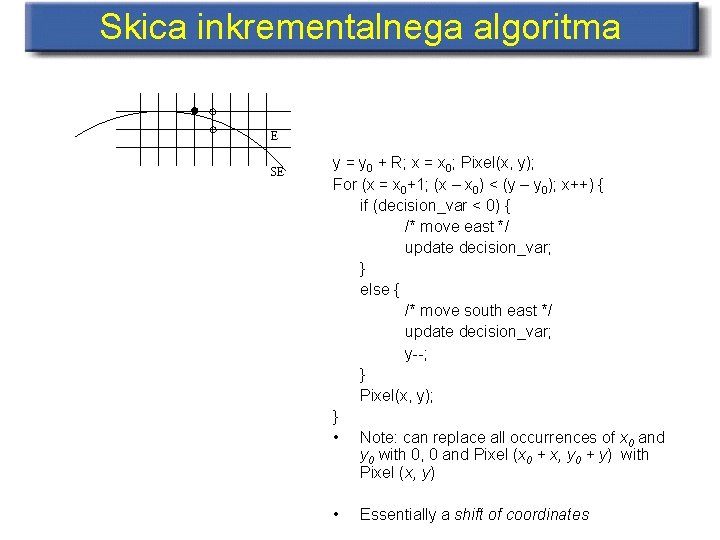
Skica inkrementalnega algoritma E SE y = y 0 + R; x = x 0; Pixel(x, y); For (x = x 0+1; (x – x 0) < (y – y 0); x++) { if (decision_var < 0) { /* move east */ update decision_var; } else { /* move south east */ update decision_var; y--; } Pixel(x, y); } • Note: can replace all occurrences of x 0 and y 0 with 0, 0 and Pixel (x 0 + x, y 0 + y) with Pixel (x, y) • Essentially a shift of coordinates

Poligoni

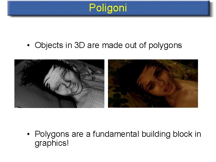
Poligoni • Objects in 3 D are made out of polygons • Polygons are a fundamental building block in graphics!

Rasterizacija poligonov • In interactive graphics, polygons rule the world • Two main reasons: – Lowest common denominator for surfaces • Can represent any surface with arbitrary accuracy • Splines, mathematical functions, volumetric isosurfaces… – Mathematical simplicity lends itself to simple, regular rendering algorithms • Like those we’re about to discuss… • Such algorithms embed well in hardware

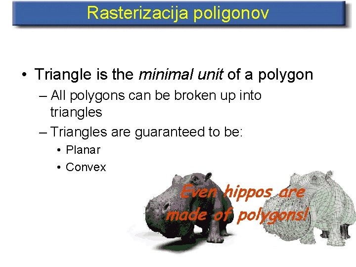
Rasterizacija poligonov • Triangle is the minimal unit of a polygon – All polygons can be broken up into triangles – Triangles are guaranteed to be: • Planar • Convex

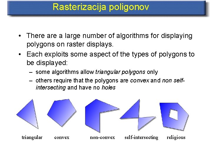
Rasterizacija poligonov • There a large number of algorithms for displaying polygons on raster displays. • Each exploits some aspect of the types of polygons to be displayed: – some algorithms allow triangular polygons only – others require that the polygons are convex and non selfintersecting and have no holes triangular convex non-convex self-intersecting religious

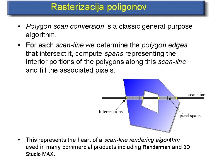
Rasterizacija poligonov • Polygon scan conversion is a classic general purpose algorithm. • For each scan-line we determine the polygon edges that intersect it, compute spans representing the interior portions of the polygons along this scan-line and fill the associated pixels. • This represents the heart of a scan-line rendering algorithm used in many commercial products including Renderman and 3 D Studio MAX.

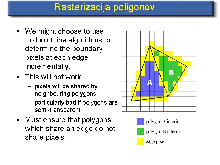
Rasterizacija poligonov • We might choose to use midpoint line algorithms to determine the boundary pixels at each edge incrementally. • This will not work: – pixels will be shared by neighbouring polygons – particularly bad if polygons are semi-transparent • Must ensure that polygons which share an edge do not share pixels.

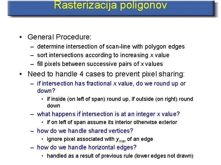
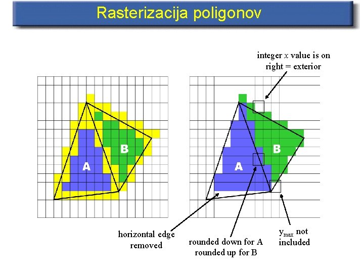
Rasterizacija poligonov • General Procedure: – determine intersection of scan-line with polygon edges – sort intersections according to increasing x value – fill pixels between successive pairs of x values • Need to handle 4 cases to prevent pixel sharing: – if intersection has fractional x value, do we round up or down? • if inside (on left of span) round up, if outside (on right) round down – what happens if intersection is at an integer x value? • if on left of span assume its interior otherwise exterior – how do we handle shared vertices? • ignore pixel associated with ymax of an edge – how do we handle horizontal edges? • handled as a result of previous rule (lower edges not drawn)

Rasterizacija poligonov integer x value is on right = exterior horizontal edge removed rounded down for A rounded up for B ymax not included

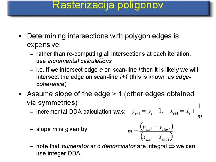
Rasterizacija poligonov • Determining intersections with polygon edges is expensive – rather than re-computing all intersections at each iteration, use incremental calculations – i. e. if we intersect edge e on scan-line i then it is likely we will intersect the edge on scan-line i+1 (this is known as edgecoherence) • Assume slope of the edge > 1 (other edges obtained via symmetries) – incremental DDA calculation was: – slope m is given by – note that numerator and denominator are integral we can use integer DDA.

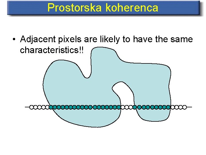
Metode rasterizacije • Makes use of the coherence properties – Spatial coherence : Except at the boundary edges, adjacent pixels are likely to have the same characteristics – Span coherence : Pixels in a scan line will be set to same values for solid shaded primitives – Scan line coherence : Pixels in the adjacent scan lines are likely to have the same characteristics • Uses intersections between area boundaries and scan lines to identify pixels that are inside the area

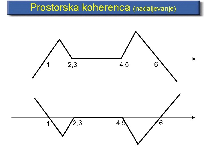
Prostorska koherenca • Adjacent pixels are likely to have the same characteristics!!

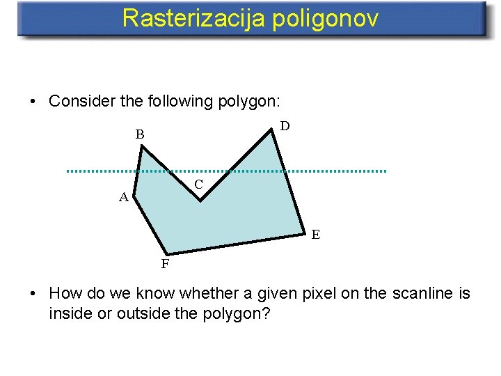
Rasterizacija poligonov • Consider the following polygon: D B C A E F • How do we know whether a given pixel on the scanline is inside or outside the polygon?

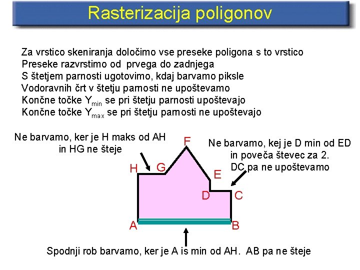
Rasterizacija poligonov Za vrstico skeniranja določimo vse preseke poligona s to vrstico Preseke razvrstimo od prvega do zadnjega S štetjem parnosti ugotovimo, kdaj barvamo piksle Vodoravnih črt v štetju parnosti ne upoštevamo Končne točke Ymin se pri štetju parnosti upoštevajo Končne točke Ymax se pri štetju parnosti ne upoštevajo Ne barvamo, ker je H maks od AH in HG ne šteje H G F Ne barvamo, kej je D min od ED in poveča števec za 2. DC pa ne upoštevamo E D A C B Spodnji rob barvamo, ker je A is min od AH. AB pa ne šteje

Barvanje poligonov • Find intersections of scanline with all polygon edges • Sort intersections by increasing x • Fill all interior pixels between pairs of intersections (odd-parity rule)

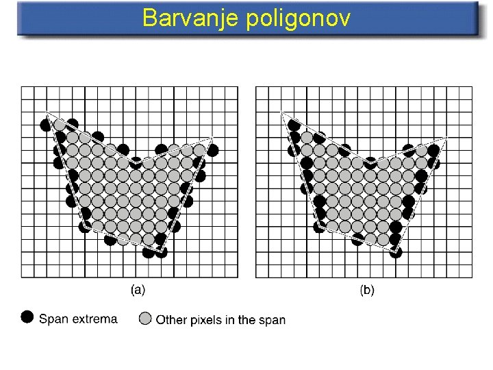
Barvanje poligonov

Prednosti metode Scan Line • The algorithm is efficient • Each pixel is visited only once • Shading algorithms could be easily integrated with this method to obtain shaded area

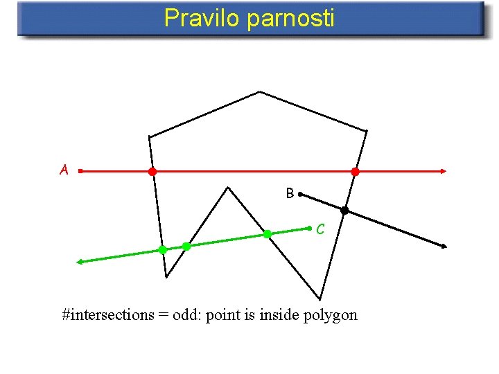
Pravilo parnosti A B C #intersections = odd: point is inside polygon

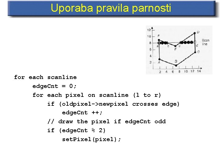
Uporaba pravila parnosti for each scanline edge. Cnt = 0; for each pixel on scanline (l to r) if (oldpixel->newpixel crosses edge) edge. Cnt ++; // draw the pixel if edge. Cnt odd if (edge. Cnt % 2) set. Pixel(pixel);

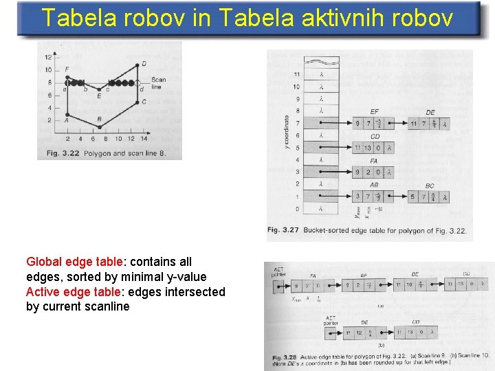
Tabela robov in Tabela aktivnih robov Global edge table: contains all edges, sorted by minimal y-value Active edge table: edges intersected by current scanline

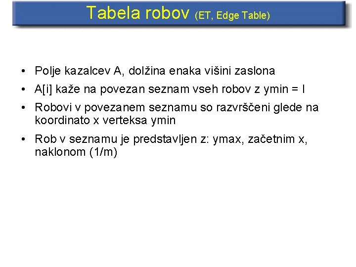
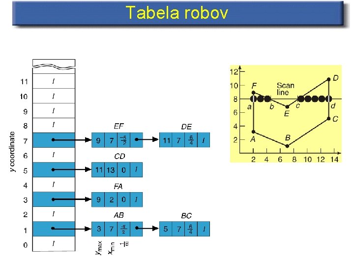
Tabela robov (ET, Edge Table) • Polje kazalcev A, dolžina enaka višini zaslona • A[i] kaže na povezan seznam vseh robov z ymin = I • Robovi v povezanem seznamu so razvrščeni glede na koordinato x verteksa ymin • Rob v seznamu je predstavljen z: ymax, začetnim x, naklonom (1/m)

Tabela robov -5 2

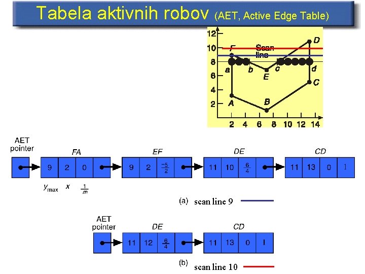
Tabela aktivnih robov – – – Povezan seznam vseh robov, ki sekajo tekočo vrstico skeniranja Seznam vedno uredimo glede na sekanje x z vrstico skeniranja Najprej dodamo vse robove iz te tabele z najmanjšim y S testom parnosti zapolnjujemo (barvamo) piksle na vrstici skeniranja Vrstico skeniranja premikamo navzgor Dodajamo vse robove iz tabele robov, pri katerih je vrednost ymin enaka vrstici skeniranja – Odstranimo vse robove iz tabele aktivnih robov, pri katerih je vrednost ymax enaka vrstici skeniranja – Posodobimo vrednosti x vrednosti presečišč vseh robov v aktivni tabeli robov in prerarvrstimo

Tabela aktivnih robov (AET, Active Edge Table) scan line 9 scan line 10

Algoritem • The scan-line algorithm uses edge-coherence and incremental integer calculations for maximum efficiency: – create an edge table (ET) which lists all edges in order to their ymin value – keep track of an active edge table (AET) which lists those edges under the current scan-line • As the scan progresses, edges are moved from the ET to the AET. • An edge remains in the AET until ymax for that edge has been reached. • At this point the edge is removed from the AET.

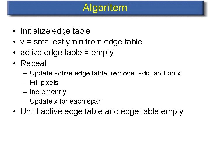
Algoritem • • Initialize edge table y = smallest ymin from edge table active edge table = empty Repeat: – – Update active edge table: remove, add, sort on x Fill pixels Increment y Update x for each span • Untill active edge table and edge table empty

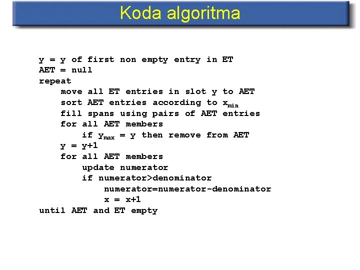
Koda algoritma y = y of first non empty entry in ET AET = null repeat move all ET entries in slot y to AET sort AET entries according to xmin fill spans using pairs of AET entries for all AET members if ymax = y then remove from AET y = y+1 for all AET members update numerator if numerator>denominator numerator=numerator-denominator x = x+1 until AET and ET empty

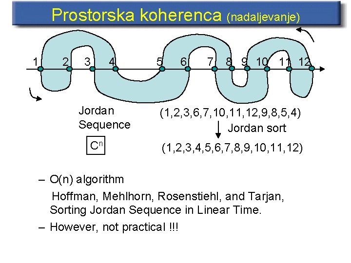
Prostorska koherenca (nadaljevanje) 1 2 3 4 Jordan Sequence Cn 5 6 7 8 9 10 11 12 (1, 2, 3, 6, 7, 10, 11, 12, 9, 8, 5, 4) Jordan sort (1, 2, 3, 4, 5, 6, 7, 8, 9, 10, 11, 12) – O(n) algorithm Hoffman, Mehlhorn, Rosenstiehl, and Tarjan, Sorting Jordan Sequence in Linear Time. – However, not practical !!!

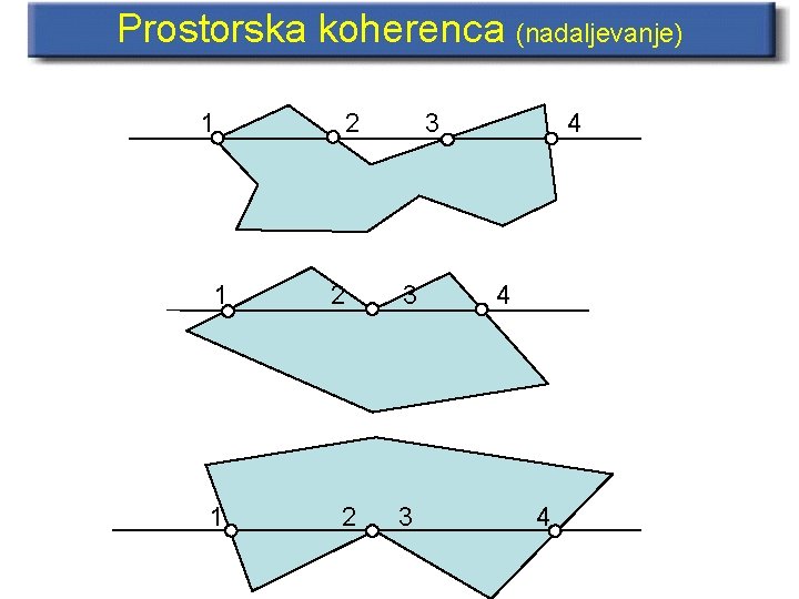
Prostorska koherenca (nadaljevanje) 1 1 1 2 2 2 3 3 3 4 4 4

Prostorska koherenca (nadaljevanje) 1 1 2, 3 4, 5 6 6

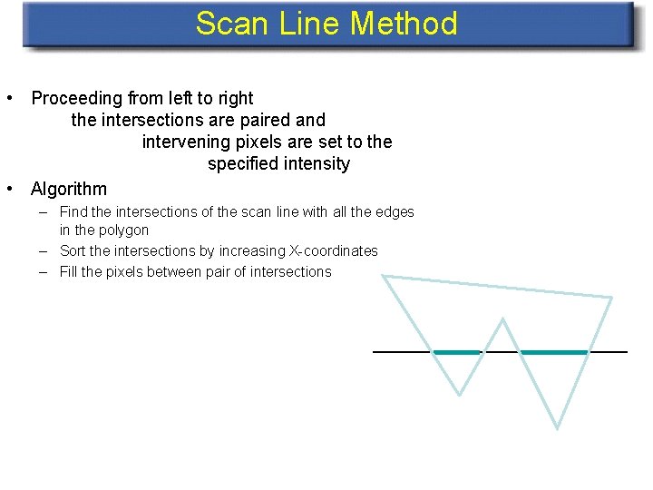
Scan Line Method • Proceeding from left to right the intersections are paired and intervening pixels are set to the specified intensity • Algorithm – Find the intersections of the scan line with all the edges in the polygon – Sort the intersections by increasing X-coordinates – Fill the pixels between pair of intersections

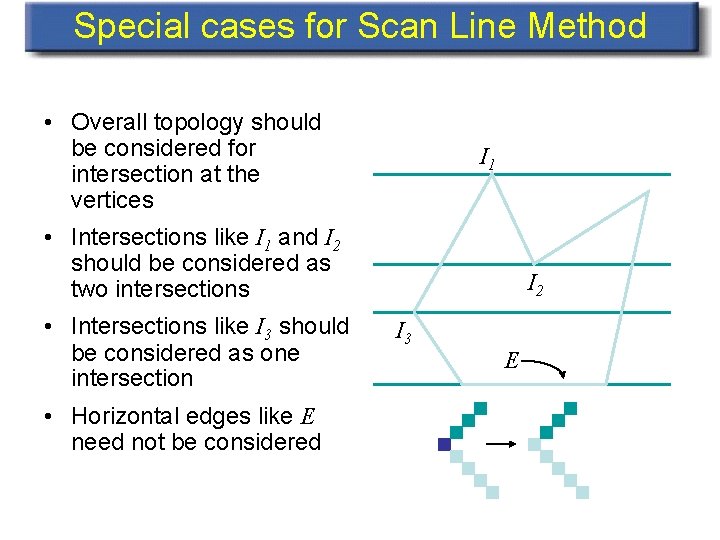
Special cases for Scan Line Method • Overall topology should be considered for intersection at the vertices I 1 • Intersections like I 1 and I 2 should be considered as two intersections • Intersections like I 3 should be considered as one intersection • Horizontal edges like E need not be considered I 2 I 3 E

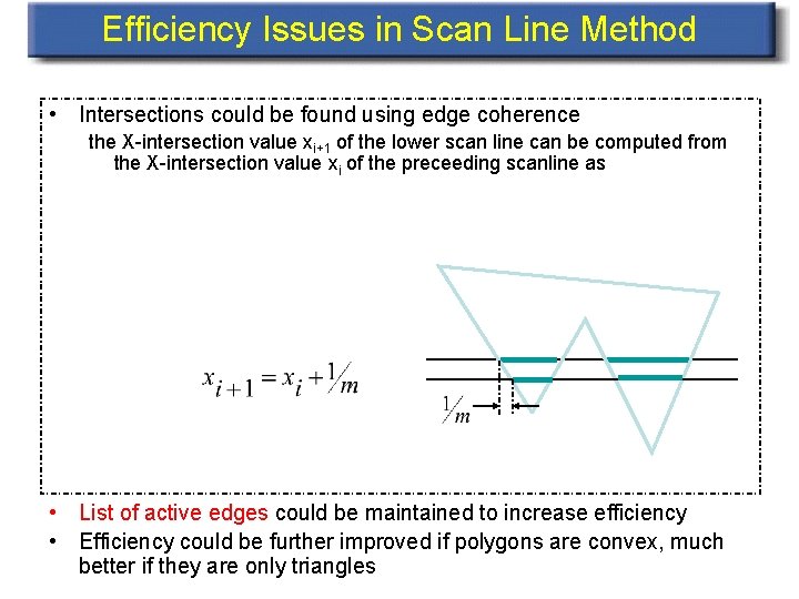
Efficiency Issues in Scan Line Method • Intersections could be found using edge coherence the X-intersection value xi+1 of the lower scan line can be computed from the X-intersection value xi of the preceeding scanline as • List of active edges could be maintained to increase efficiency • Efficiency could be further improved if polygons are convex, much better if they are only triangles

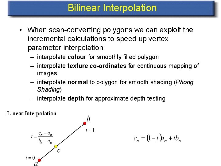
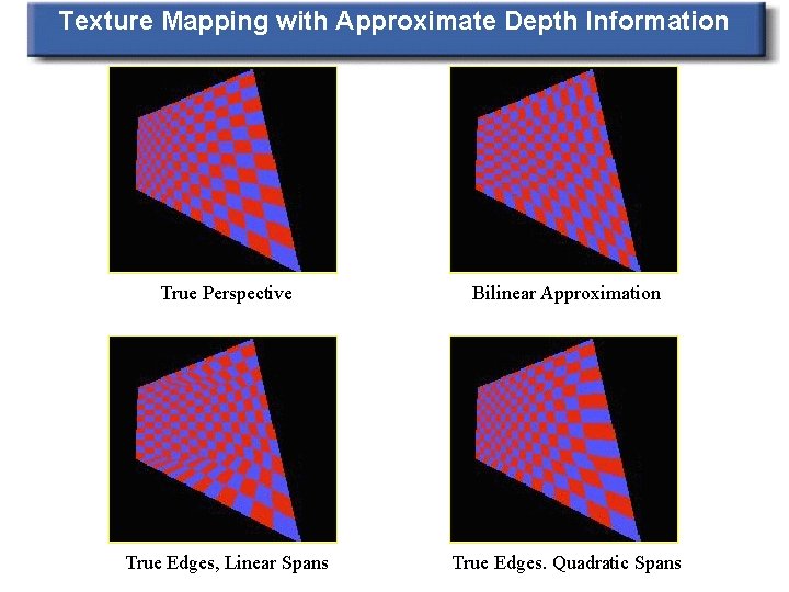
Bilinear Interpolation • When scan-converting polygons we can exploit the incremental calculations to speed up vertex parameter interpolation: – interpolate colour for smoothly filled polygon – interpolate texture co-ordinates for continuous mapping of images – interpolate normal to polygon for smooth shading (Phong Shading) – interpolate depth for approximate depth testing Linear Interpolation

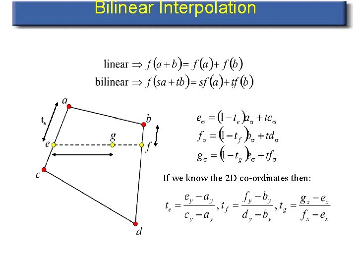
Bilinear Interpolation te If we know the 2 D co-ordinates then:

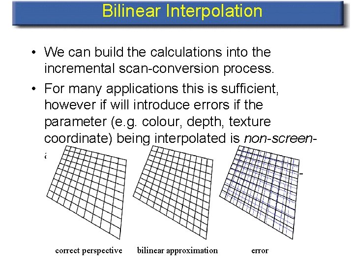
Bilinear Interpolation • We can build the calculations into the incremental scan-conversion process. • For many applications this is sufficient, however if will introduce errors if the parameter (e. g. colour, depth, texture coordinate) being interpolated is non-screenaffine. – distance from viewer, and therefore texture coordinates are non-screen affine: correct perspective bilinear approximation error

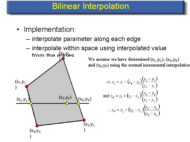
Bilinear Interpolation • Implementation: – interpolate parameter along each edge – interpolate within space using interpolated value (x 2, y 2 from the edges ) We assume we have determined (x , y ), (x L L R, y. R) and (x. P, y. P) using the normal incremental interpolation (x 1, y 1 ) (x. P, y. P) (x. L, y. L) (x 4, y 4 ) (x. R, y. R) (x 3, y 3 )

Texture Mapping with Approximate Depth Information True Perspective Bilinear Approximation True Edges, Linear Spans True Edges. Quadratic Spans

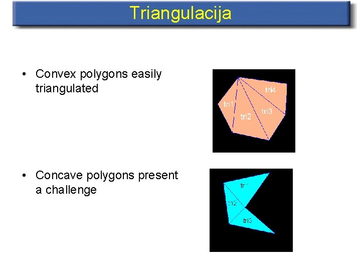
Triangulacija • Convex polygons easily triangulated • Concave polygons present a challenge

Rasterizacija trikotnikov • Interactive graphics hardware commonly uses edge walking or edge equation techniques for rasterizing triangles

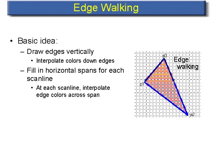
Edge Walking • Basic idea: – Draw edges vertically • Interpolate colors down edges – Fill in horizontal spans for each scanline • At each scanline, interpolate edge colors across span

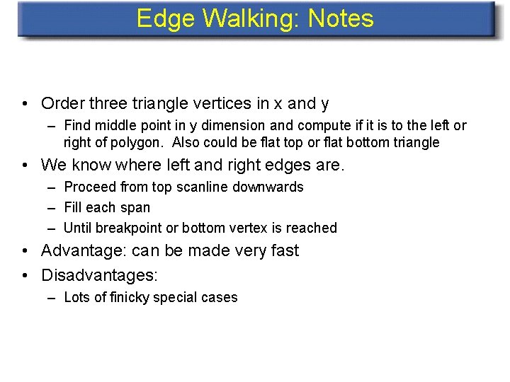
Edge Walking: Notes • Order three triangle vertices in x and y – Find middle point in y dimension and compute if it is to the left or right of polygon. Also could be flat top or flat bottom triangle • We know where left and right edges are. – Proceed from top scanline downwards – Fill each span – Until breakpoint or bottom vertex is reached • Advantage: can be made very fast • Disadvantages: – Lots of finicky special cases

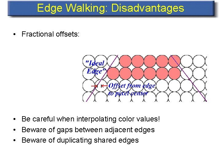
Edge Walking: Disadvantages • Fractional offsets: • Be careful when interpolating color values! • Beware of gaps between adjacent edges • Beware of duplicating shared edges

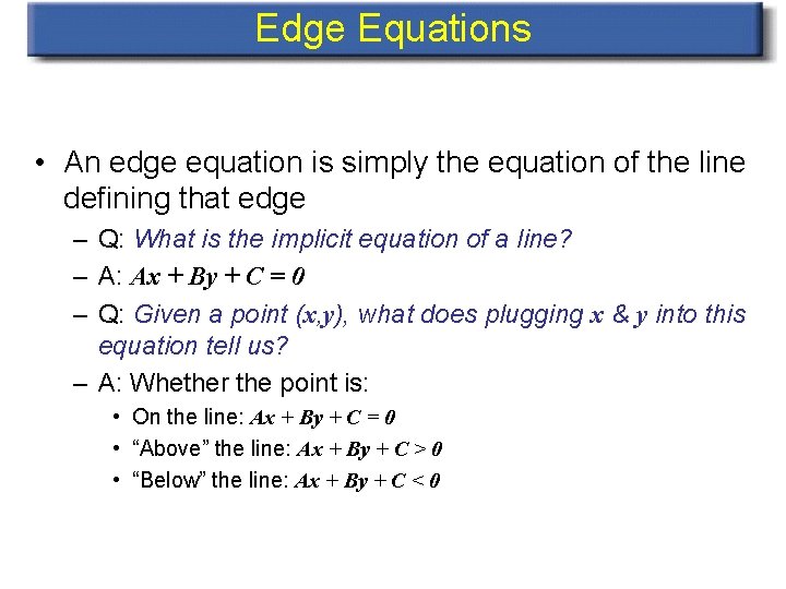
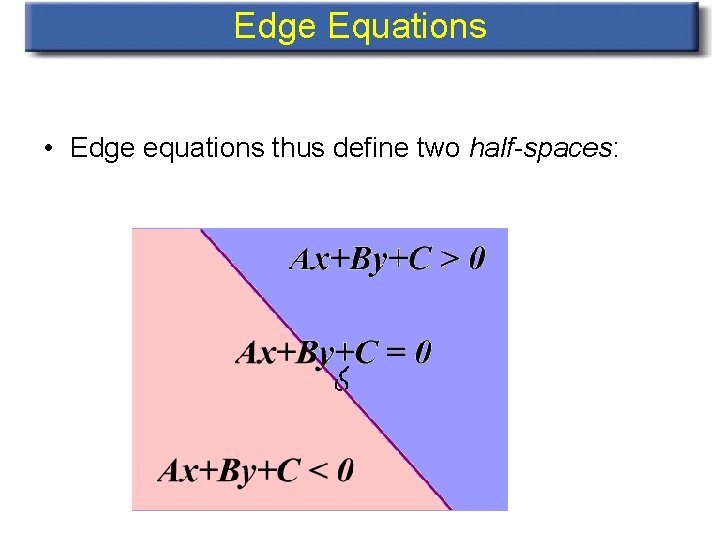
Edge Equations • An edge equation is simply the equation of the line defining that edge – Q: What is the implicit equation of a line? – A: Ax + By + C = 0 – Q: Given a point (x, y), what does plugging x & y into this equation tell us? – A: Whether the point is: • On the line: Ax + By + C = 0 • “Above” the line: Ax + By + C > 0 • “Below” the line: Ax + By + C < 0

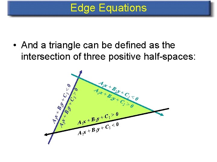
Edge Equations • Edge equations thus define two half-spaces:

Edge Equations • And a triangle can be defined as the intersection of three positive half-spaces: >0 3 +C 3 y +B A 3 x +B 3 y +C 3 <0 A 2 x +B +B 2 y 2 y +C +C 2 >0 C 1 + By A 1 x + 1 C 1 < 0 + y B A 1 x + 1 2 <0 >0

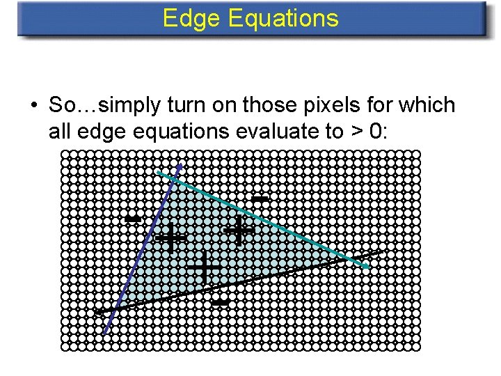
Edge Equations • So…simply turn on those pixels for which all edge equations evaluate to > 0: -+ + +-

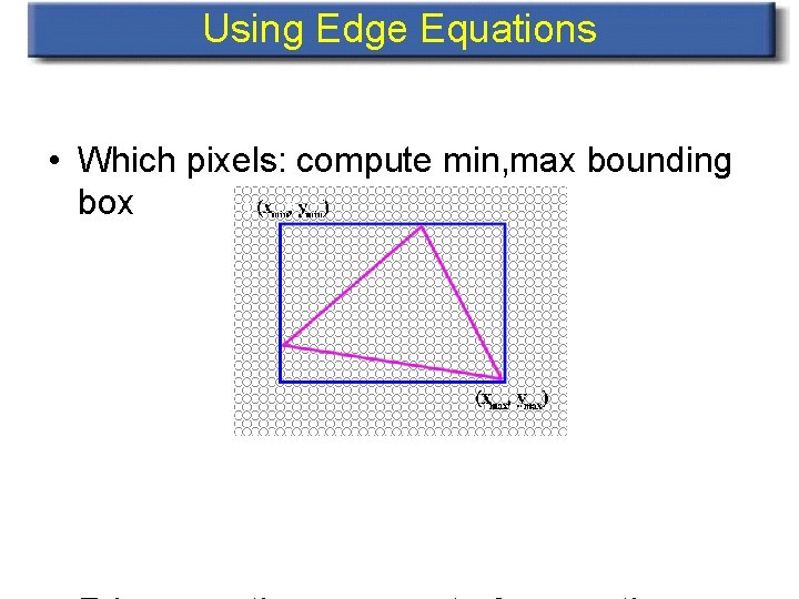
Using Edge Equations • Which pixels: compute min, max bounding box

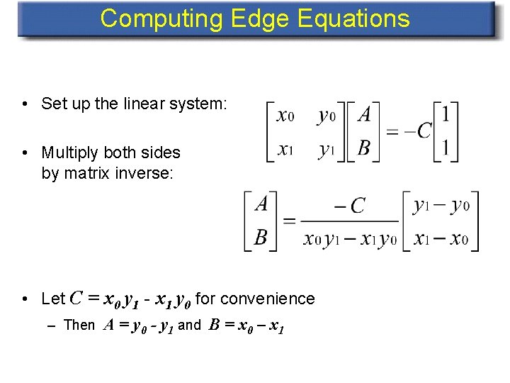
Computing Edge Equations • Want to calculate A, B, C for each edge from (x 1, y 1) and (x 2, y 2) • Treat it as a linear system: Ax 1 + By 1 + C = 0 Ax 2 + By 2 + C = 0 • Notice: two equations, three unknowns • What can we solve? • Goal: solve for A & B in terms of C

Computing Edge Equations • Set up the linear system: • Multiply both sides by matrix inverse: • Let C = x 0 y 1 - x 1 y 0 for convenience – Then A = y 0 - y 1 and B = x 0 – x 1

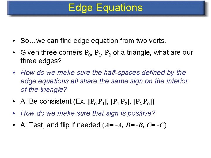
Edge Equations • So…we can find edge equation from two verts. • Given three corners P 0, P 1, P 2 of a triangle, what are our three edges? • How do we make sure the half-spaces defined by the edge equations all share the same sign on the interior of the triangle? • A: Be consistent (Ex: [P 0 P 1], [P 1 P 2], [P 2 P 0]) • How do we make sure that sign is positive? • A: Test, and flip if needed (A= -A, B= -B, C= -C)

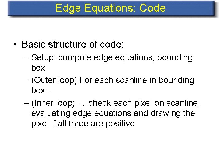
Edge Equations: Code • Basic structure of code: – Setup: compute edge equations, bounding box – (Outer loop) For each scanline in bounding box. . . – (Inner loop) …check each pixel on scanline, evaluating edge equations and drawing the pixel if all three are positive

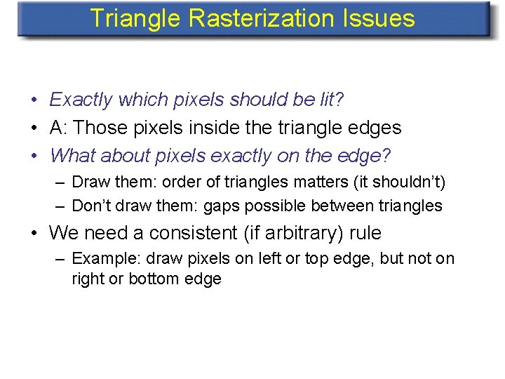
Triangle Rasterization Issues • Exactly which pixels should be lit? • A: Those pixels inside the triangle edges • What about pixels exactly on the edge? – Draw them: order of triangles matters (it shouldn’t) – Don’t draw them: gaps possible between triangles • We need a consistent (if arbitrary) rule – Example: draw pixels on left or top edge, but not on right or bottom edge

Polygon filling • Simplest method to fill a polygonal area is to test every pixel in the raster to see if it lies inside the polygon. • There are two methods to make an inside check – even-odd test – winding number test • Bounding boxes can be used to improve performance

Filling Regions • Color all pixels in a given region • Region = – All pixels of a certain color (pixel-defined regions) – All pixels within a distance of another pixel’ – All pixels within some given polygon (polygondefined region)

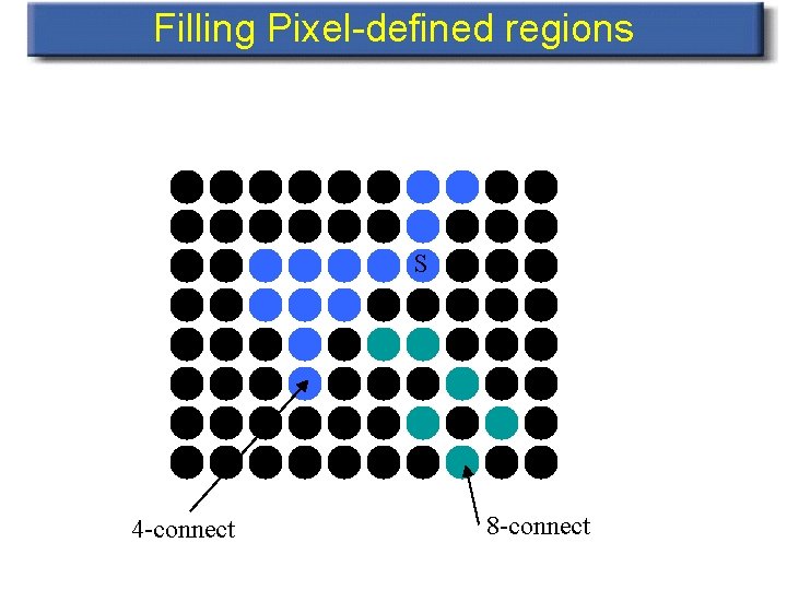
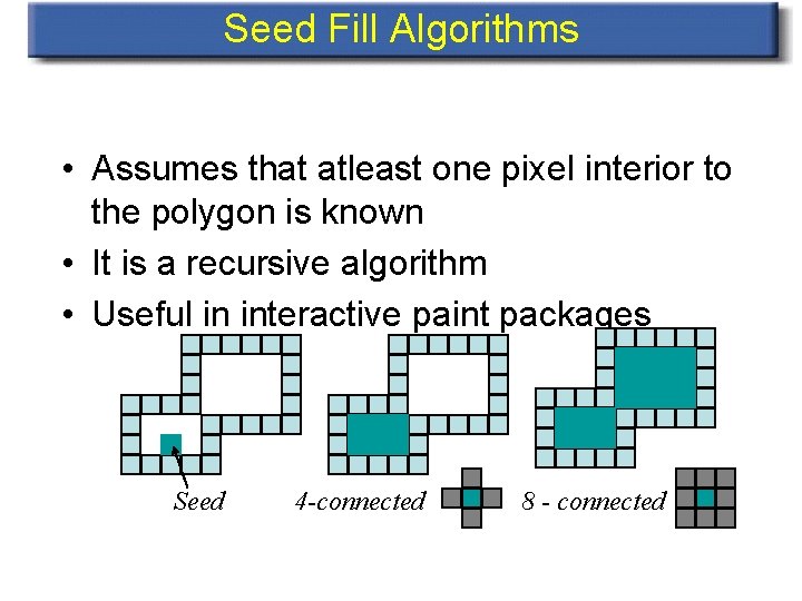
Filling Pixel-defined regions • Region R is the set of all pixels having color C that are “connected” to a given pixel S • Connected = there is path of adjacent pixels • Adjacent – 4 -adjacent – 8 -adjacent

Filling Pixel-defined regions S 4 -connect 8 -connect

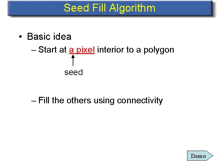
Seed Fill Algorithm • Basic idea – Start at a pixel interior to a polygon seed – Fill the others using connectivity Demo

Seed Fill Algorithms • Assumes that atleast one pixel interior to the polygon is known • It is a recursive algorithm • Useful in interactive paint packages Seed 4 -connected 8 - connected

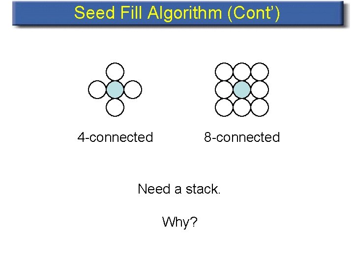
Seed Fill Algorithm (Cont’) 4 -connected 8 -connected Need a stack. Why?

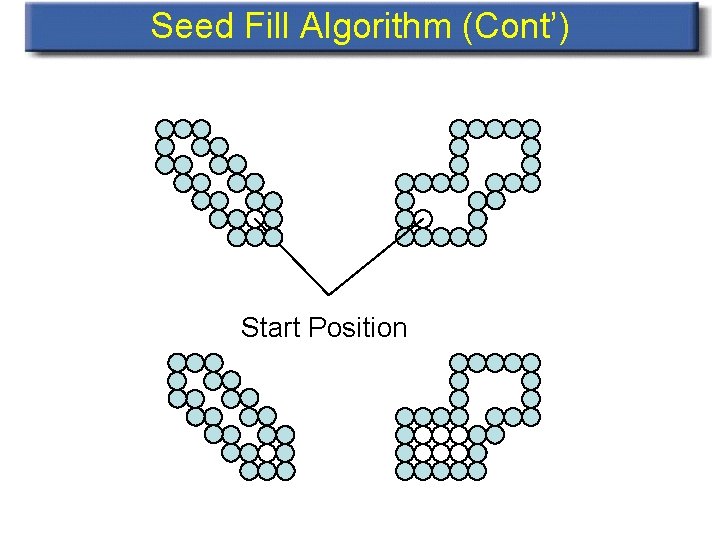
Seed Fill Algorithm (Cont’) Start Position

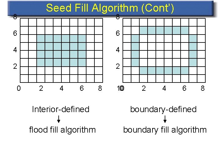
Seed Fill Algorithm (Cont’) 8 8 6 6 4 4 2 2 0 2 4 6 8 10 0 2 4 6 8 Interior-defined boundary-defined flood fill algorithm boundary fill algorithm 1

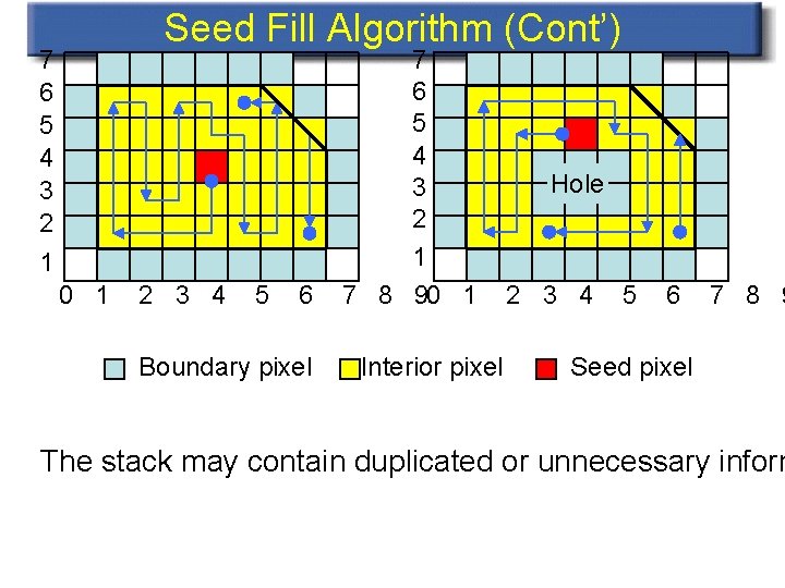
Seed Fill Algorithm (Cont’) 7 6 5 4 3 2 1 0 1 2 3 4 5 6 Boundary pixel 7 6 5 4 3 2 1 7 8 90 1 Interior pixel Hole 2 3 4 5 6 7 8 9 Seed pixel The stack may contain duplicated or unnecessary inform

Scan Line Seed Fill Scan Line conversion + Seed filling Shani, U. , “Filling Regions in Binary Raster Images A Graph-Theoretic Approach”, Computer Graphics 14, (1981), 321 -327

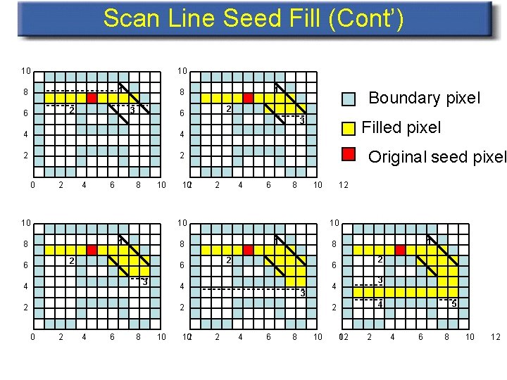
Scan Line Seed Fill (Cont’) 10 10 1 8 2 6 3 4 2 2 2 4 6 8 10 10 12 0 Boundary pixel 2 6 4 0 1 8 3 Filled pixel Original seed pixel 2 4 6 8 10 10 1 8 2 6 3 2 4 6 8 10 12 0 3 4 3 2 0 2 6 4 2 1 8 2 6 4 12 2 4 6 8 10 5 4 2 0 12 2 4 6 8 10 12

Filling Pixel-defined regions • Recursive flood-fill – If a pixel is part of the region, switch its color – Apply the same procedure to each neighbor • Neighbor = 4 -connect or 8 -connect

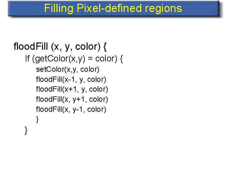
Filling Pixel-defined regions flood. Fill (x, y, color) { If (get. Color(x, y) = color) { set. Color(x, y, color) flood. Fill(x-1, y, color) flood. Fill(x+1, y, color) flood. Fill(x, y+1, color) flood. Fill(x, y-1, color) } }

Filling Symbolic Regions • If we have a description of the region (e. g. polygon), filling might be more efficient! • Scan-line fill of polygon – For each scan line, find intersections with the polygon – Fill in the spans – Go to next scanline

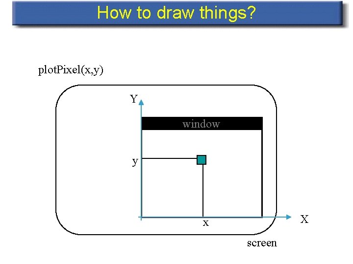
How to draw things? • Given: window on the screen • Graphics API (e. g. Open. GL) has something of the form: plot. Pixel(int x, int y)

How to draw things? plot. Pixel(x, y) Y window y X x screen

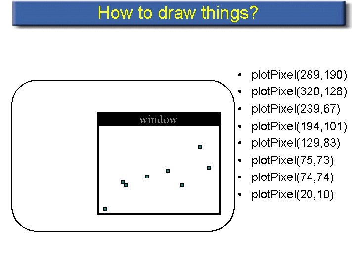
How to draw things? window • • plot. Pixel(289, 190) plot. Pixel(320, 128) plot. Pixel(239, 67) plot. Pixel(194, 101) plot. Pixel(129, 83) plot. Pixel(75, 73) plot. Pixel(74, 74) plot. Pixel(20, 10)

Why is this impractical? • Coordinates are expressed in screen space, but objects live in (3 D) world space • Resizing window implies we have to change coordinates of objects to be drawn • We want to make a separation between: – values to describe geometrical objects – values needed to draw these objects on the screen

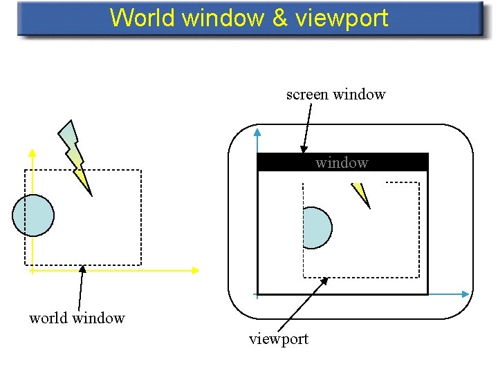
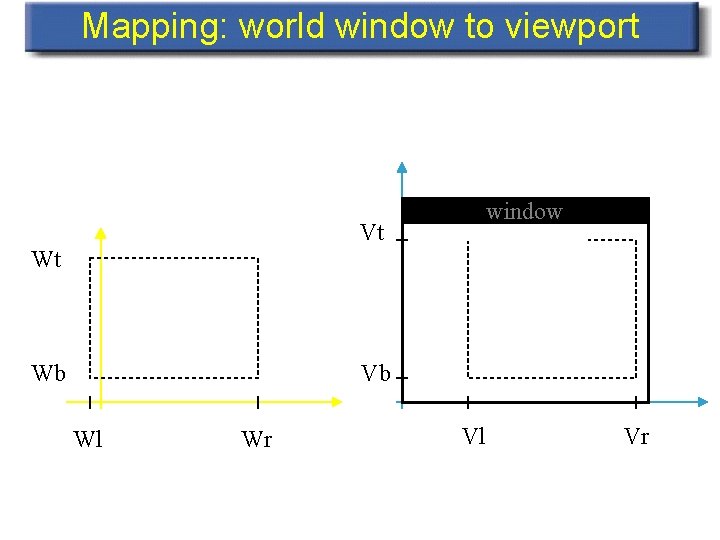
World window & viewport • World window: specifies what part of the world should be drawn • Viewport: rectangular area in the screen window in which we will draw

World window & viewport screen window world window viewport

Mapping: world window to viewport window Vt Wt Wb Vb Wl Wr Vl Vr

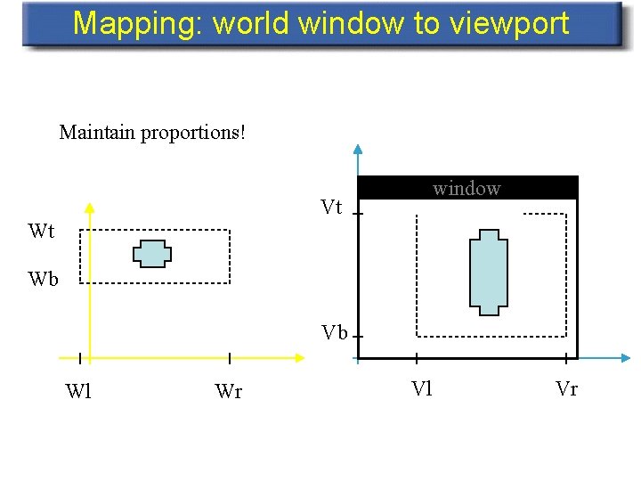
Mapping: world window to viewport Maintain proportions! window Vt Wt Wb Vb Wl Wr Vl Vr

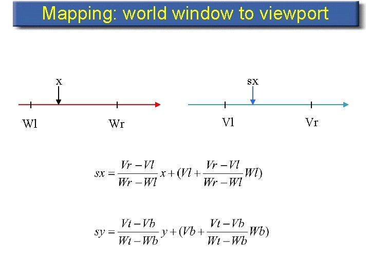
Mapping: world window to viewport x Wl sx Wr Vl Vr

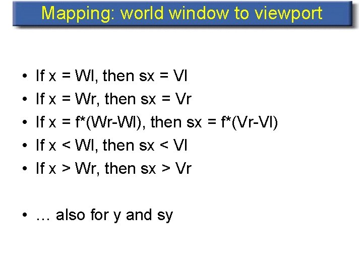
Mapping: world window to viewport • • • If x = Wl, then sx = Vl If x = Wr, then sx = Vr If x = f*(Wr-Wl), then sx = f*(Vr-Vl) If x < Wl, then sx < Vl If x > Wr, then sx > Vr • … also for y and sy

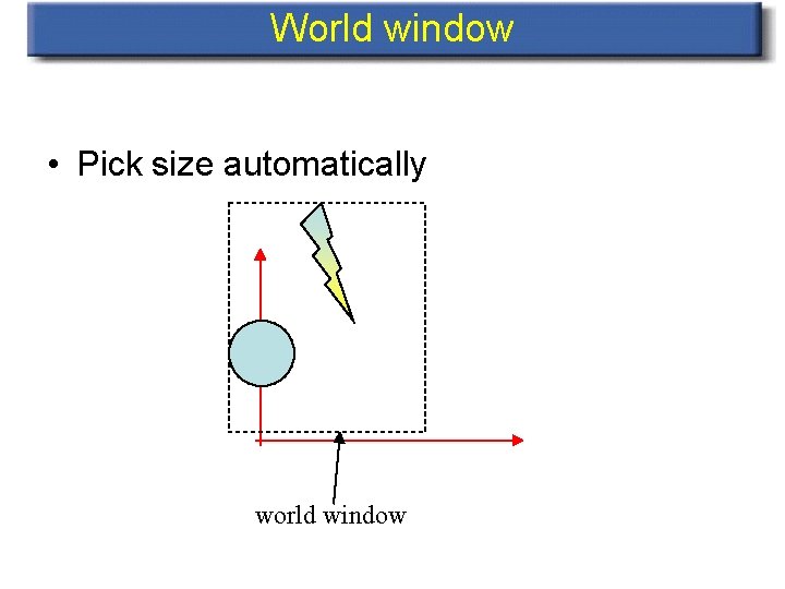
World window • Pick size automatically world window

Automatic setting to preserve aspect ratio & center window H Aspect ratio R W R > W/H

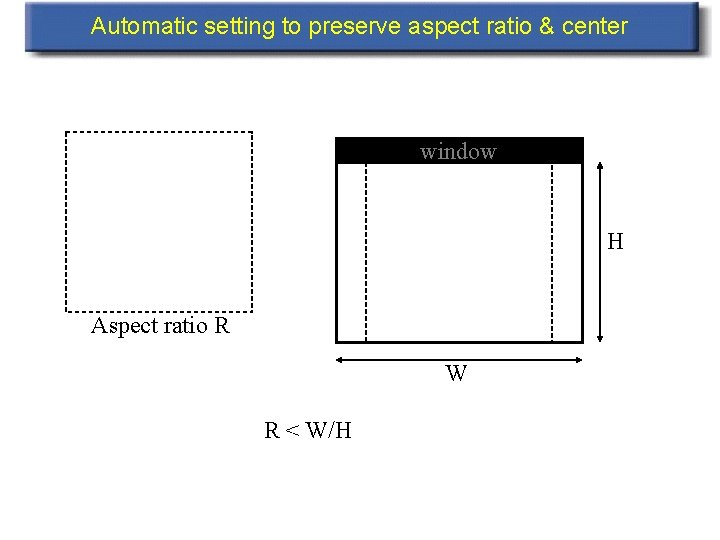
Automatic setting to preserve aspect ratio & center window H Aspect ratio R W R < W/H