Algorithms Searching and Sorting Algorithm Efficiency 1 Efficiency

Algorithms Searching and Sorting Algorithm Efficiency 1

Efficiency l A computer program should be totally correct, but it should also l l l execute as quickly as possible (time-efficiency) use memory wisely (storage-efficiency) How do we compare programs (or algorithms in general) with respect to execution time? l l l various computers run at different speeds due to different processors compilers optimize code before execution the same algorithm can be written differently depending on the programming language used 2

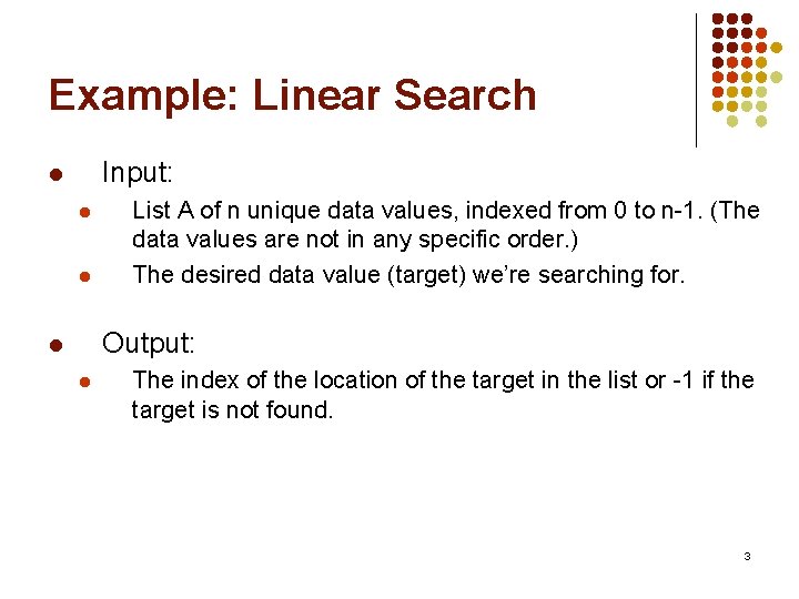
Example: Linear Search Input: l l l List A of n unique data values, indexed from 0 to n-1. (The data values are not in any specific order. ) The desired data value (target) we’re searching for. Output: l l The index of the location of the target in the list or -1 if the target is not found. 3

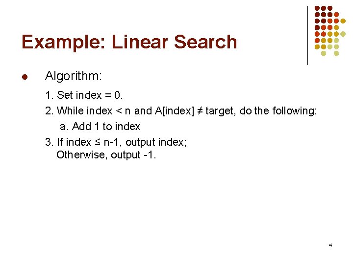
Example: Linear Search l Algorithm: 1. Set index = 0. 2. While index < n and A[index] ≠ target, do the following: a. Add 1 to index 3. If index ≤ n-1, output index; Otherwise, output -1. 4

Example: Linear Search index 0 no index < n and A[index] ≠ target yes index + 1 Algorithm: yes index ≤ n-1 no -1 1. Set index = 0. 2. While index < n and A[index] ≠ target, do the following: a. Add 1 to index 3. If index ≤ n-1, output index; Otherwise, output -1. 5

Example: Linear Search index 0 yes De. Morgan’s Law: index >= n or A[index] = target not (A and B) = (not A) or (not B) no index + 1 Algorithm: yes index ≤ n-1 no -1 1. Set index = 0. 2. While index < n and A[index] ≠ target, do the following: a. Add 1 to index 3. If index ≤ n-1, output index; Otherwise, output -1. 6

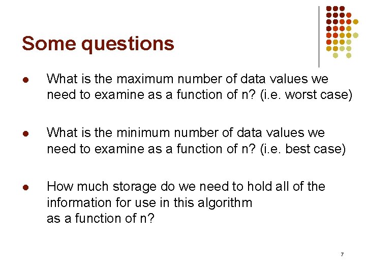
Some questions l What is the maximum number of data values we need to examine as a function of n? (i. e. worst case) l What is the minimum number of data values we need to examine as a function of n? (i. e. best case) l How much storage do we need to hold all of the information for use in this algorithm as a function of n? 7

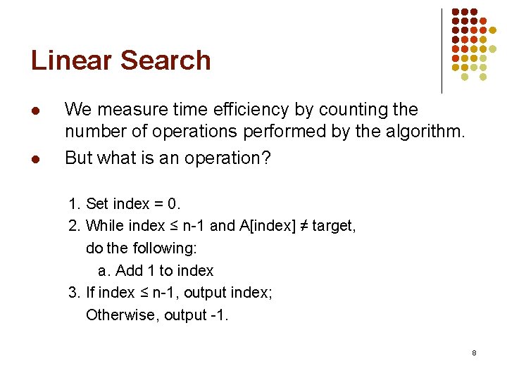
Linear Search l l We measure time efficiency by counting the number of operations performed by the algorithm. But what is an operation? 1. Set index = 0. 2. While index ≤ n-1 and A[index] ≠ target, do the following: a. Add 1 to index 3. If index ≤ n-1, output index; Otherwise, output -1. 8

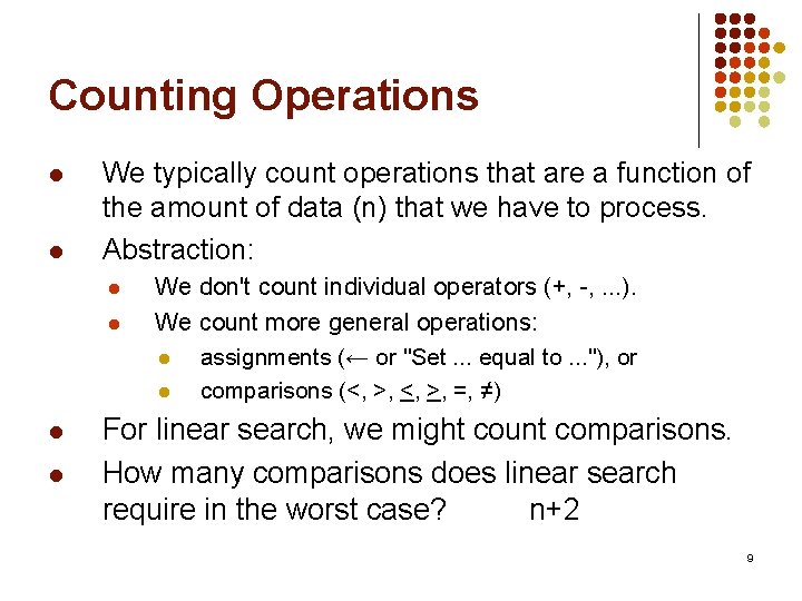
Counting Operations l l We typically count operations that are a function of the amount of data (n) that we have to process. Abstraction: l l We don't count individual operators (+, -, . . . ). We count more general operations: l assignments (← or "Set. . . equal to. . . "), or l comparisons (<, >, =, ≠) For linear search, we might count comparisons. How many comparisons does linear search require in the worst case? n+2 9

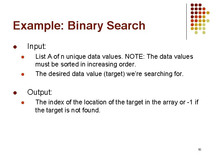
Example: Binary Search Input: l l l List A of n unique data values. NOTE: The data values must be sorted in increasing order. The desired data value (target) we’re searching for. Output: l l The index of the location of the target in the array or -1 if the target is not found. 10

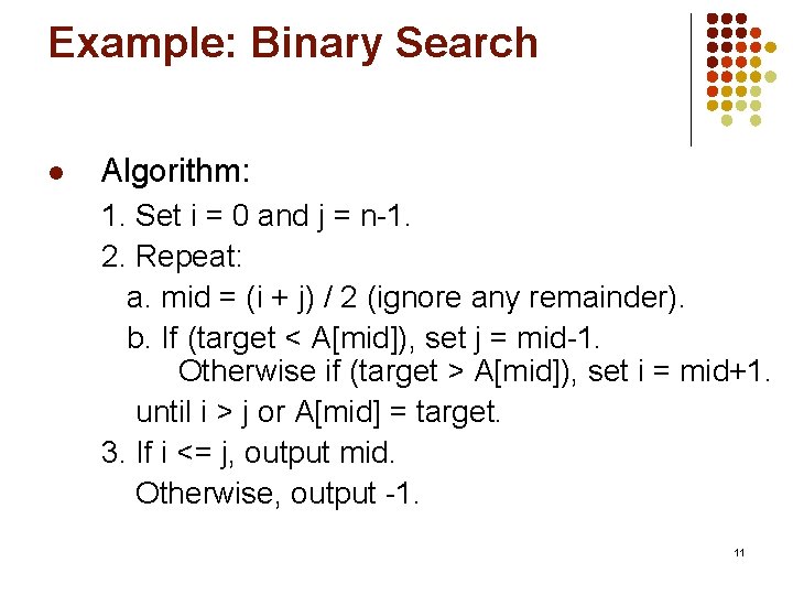
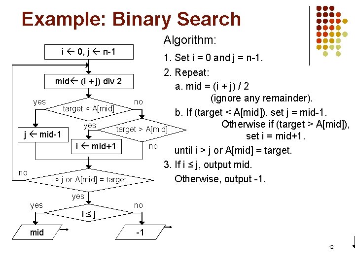
Example: Binary Search l Algorithm: 1. Set i = 0 and j = n-1. 2. Repeat: a. mid = (i + j) / 2 (ignore any remainder). b. If (target < A[mid]), set j = mid-1. Otherwise if (target > A[mid]), set i = mid+1. until i > j or A[mid] = target. 3. If i <= j, output mid. Otherwise, output -1. 11

Example: Binary Search Algorithm: i 0, j n-1 1. Set i = 0 and j = n-1. 2. Repeat: mid (i + j) div 2 a. mid = (i + j) / 2 (ignore any remainder). yes no target < A[mid] b. If (target < A[mid]), set j = mid-1. Otherwise if (target > A[mid]), yes target > A[mid] j mid-1 set i = mid+1. no i mid+1 until i > j or A[mid] = target. 3. If i ≤ j, output mid. no i > j or A[mid] = target Otherwise, output -1. yes mid i ≤ j no -1 12

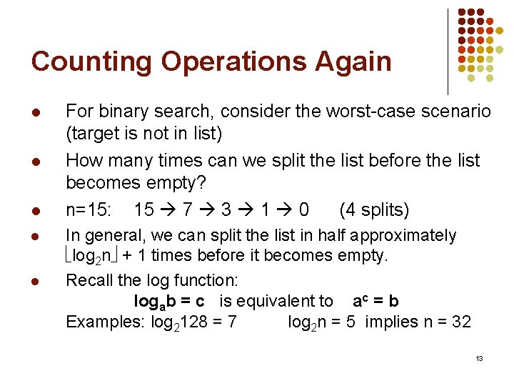
Counting Operations Again l l l For binary search, consider the worst-case scenario (target is not in list) How many times can we split the list before the list becomes empty? n=15: 15 7 3 1 0 (4 splits) In general, we can split the list in half approximately log 2 n + 1 times before it becomes empty. Recall the log function: logab = c is equivalent to ac = b Examples: log 2128 = 7 log 2 n = 5 implies n = 32 13

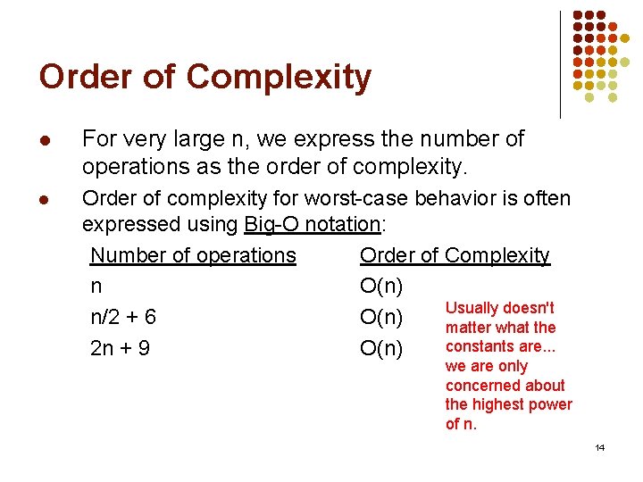
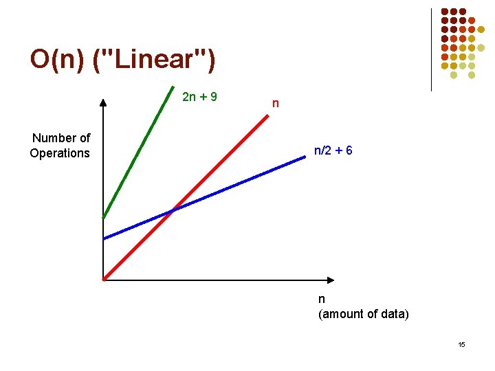
Order of Complexity l For very large n, we express the number of operations as the order of complexity. l Order of complexity for worst-case behavior is often expressed using Big-O notation: Number of operations Order of Complexity n O(n) Usually doesn't n/2 + 6 O(n) matter what the constants are. . . 2 n + 9 O(n) we are only concerned about the highest power of n. 14

O(n) ("Linear") 2 n + 9 Number of Operations n n/2 + 6 n (amount of data) 15

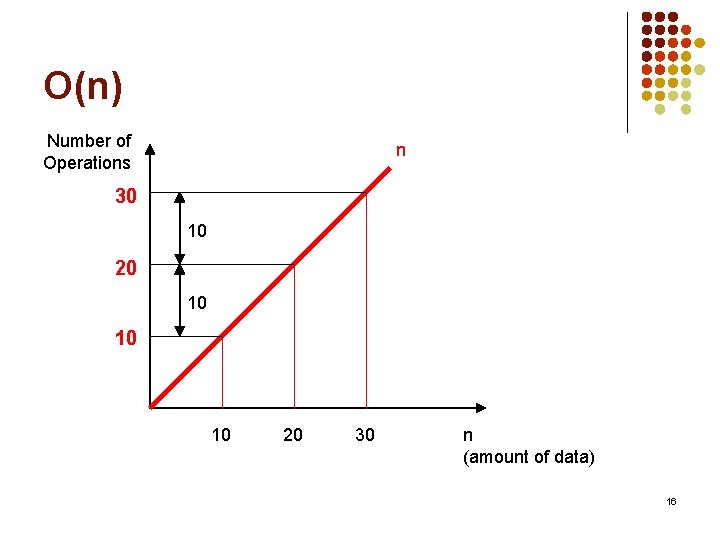
O(n) Number of Operations n 30 10 20 10 10 10 20 30 n (amount of data) 16

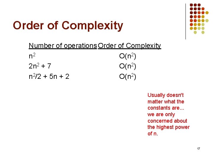
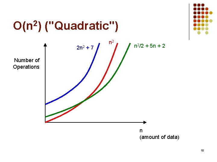
Order of Complexity Number of operations Order of Complexity n 2 O(n 2) 2 n 2 + 7 O(n 2) n 2/2 + 5 n + 2 O(n 2) Usually doesn't matter what the constants are. . . we are only concerned about the highest power of n. 17

O(n 2) ("Quadratic") 2 n 2 + 7 n 2/2 + 5 n + 2 Number of Operations n (amount of data) 18

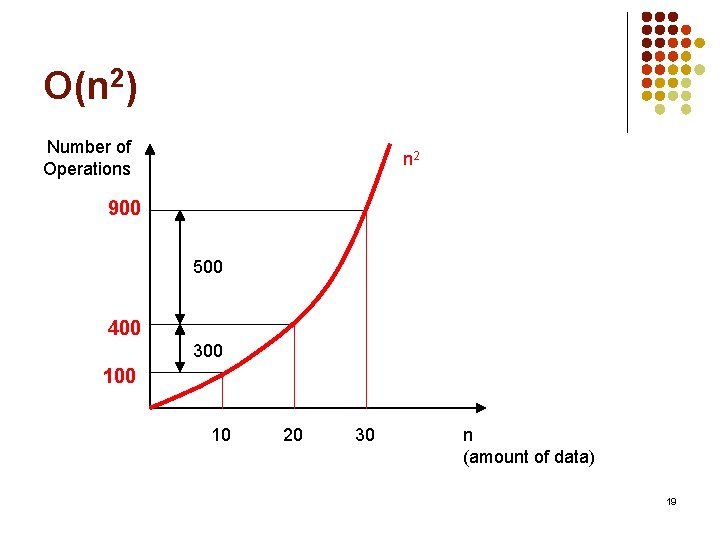
O(n 2) Number of Operations n 2 900 500 400 300 10 20 30 n (amount of data) 19

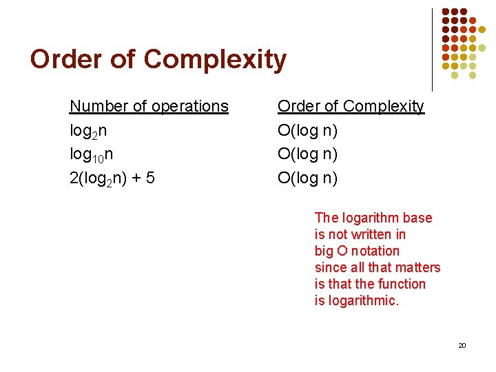
Order of Complexity Number of operations log 2 n log 10 n 2(log 2 n) + 5 Order of Complexity O(log n) The logarithm base is not written in big O notation since all that matters is that the function is logarithmic. 20

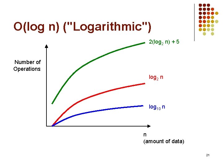
O(log n) ("Logarithmic") 2(log 2 n) + 5 Number of Operations log 2 n log 10 n n (amount of data) 21

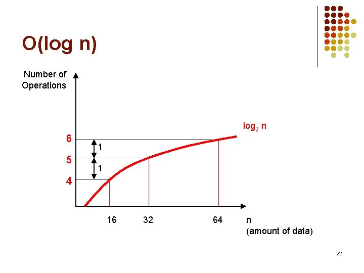
O(log n) Number of Operations log 2 n 6 5 1 1 4 16 32 64 n (amount of data) 22

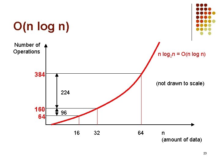
O(n log n) Number of Operations n log 2 n = O(n log n) 384 (not drawn to scale) 224 160 64 96 16 32 64 n (amount of data) 23

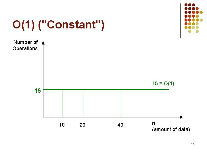
O(1) ("Constant") Number of Operations 15 = O(1) 15 10 20 40 n (amount of data) 24

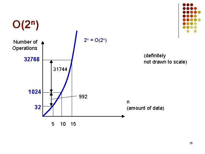
O(2 n) 2 n = O(2 n) Number of Operations (definitely not drawn to scale) 32768 31744 1024 992 32 5 n (amount of data) 10 15 25

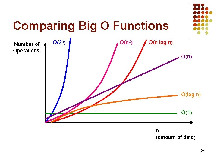
Comparing Big O Functions Number of Operations O(2 n) O(n 2) O(n log n) O(log n) O(1) n (amount of data) 26

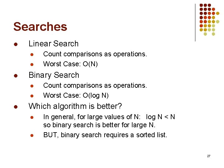
Searches l Linear Search l l l Binary Search l l l Count comparisons as operations. Worst Case: O(N) Count comparisons as operations. Worst Case: O(log N) Which algorithm is better? l l In general, for large values of N: log N < N so binary search is better for large N. BUT, binary search requires a sorted list. 27

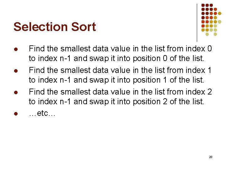
Selection Sort l l Find the smallest data value in the list from index 0 to index n-1 and swap it into position 0 of the list. Find the smallest data value in the list from index 1 to index n-1 and swap it into position 1 of the list. Find the smallest data value in the list from index 2 to index n-1 and swap it into position 2 of the list. …etc… 28

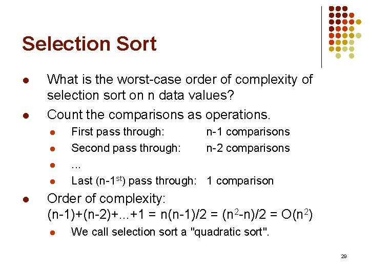
Selection Sort l l What is the worst-case order of complexity of selection sort on n data values? Count the comparisons as operations. l l l First pass through: n-1 comparisons Second pass through: n-2 comparisons. . . Last (n-1 st) pass through: 1 comparison Order of complexity: (n-1)+(n-2)+. . . +1 = n(n-1)/2 = (n 2 -n)/2 = O(n 2) l We call selection sort a "quadratic sort". 29

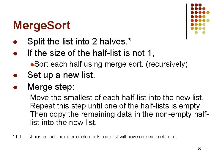
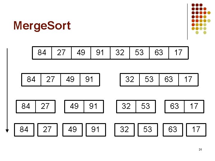
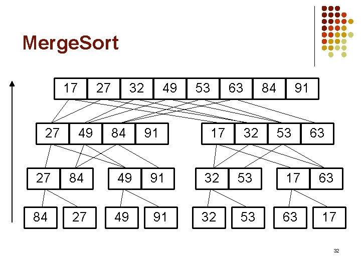
Merge. Sort l l Split the list into 2 halves. * If the size of the half-list is not 1, l. Sort each half using merge sort. (recursively) l l Set up a new list. Merge step: Move the smallest of each half-list into the new list. Repeat this step until one of the half-lists is empty. Then copy the remaining data in the non-empty halflist into the new list. *If the list has an odd number of elements, one list will have one extra element. 30

Merge. Sort 84 84 27 27 49 49 91 91 32 53 32 63 53 17 63 17 84 27 49 91 32 53 63 17 31

Merge. Sort 17 27 27 49 32 84 49 91 53 63 17 84 32 91 53 63 27 84 49 91 32 53 17 63 84 27 49 91 32 53 63 17 32

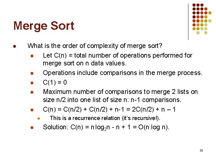
Merge Sort l What is the order of complexity of merge sort? l Let C(n) = total number of operations performed for merge sort on n data values. l Operations include comparisons in the merge process. l C(1) = 0 l Maximum number of comparisons to merge 2 lists on size n/2 into one list of size n: n-1 comparisons. l C(n) = C(n/2) + n-1 = 2 C(n/2) + n – 1 l l This is a recurrence relation (it’s recursive!). Solution: C(n) = n log 2 n - n + 1 = O(n log n). 33

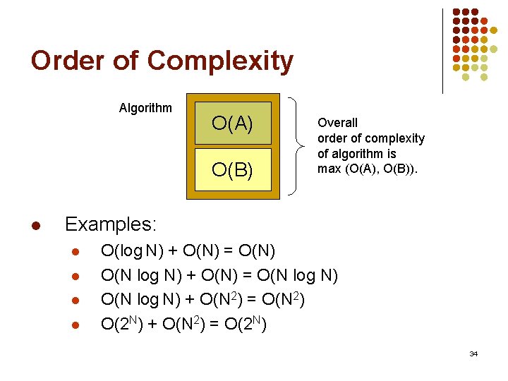
Order of Complexity Algorithm O(A) O(B) l Overall order of complexity of algorithm is max (O(A), O(B)). Examples: l l O(log N) + O(N) = O(N) O(N log N) + O(N) = O(N log N) + O(N 2) = O(N 2) O(2 N) + O(N 2) = O(2 N) 34

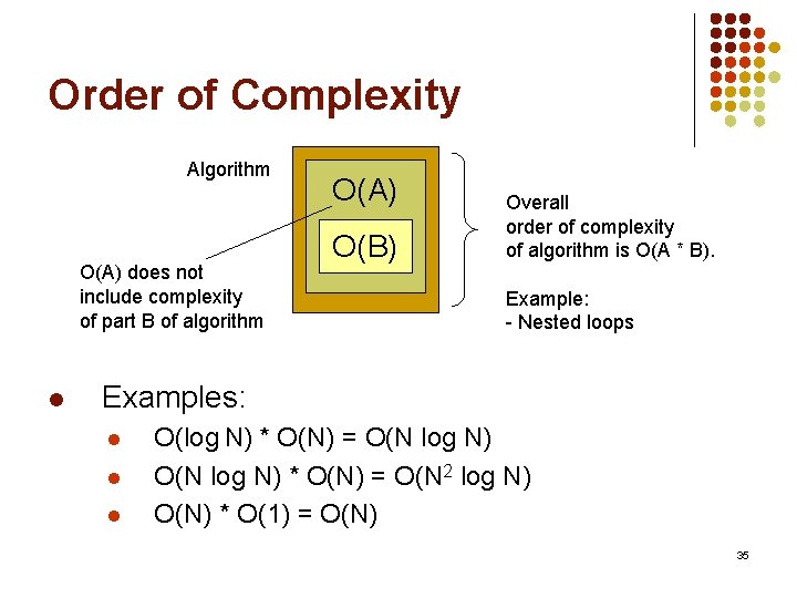
Order of Complexity Algorithm O(A) does not include complexity of part B of algorithm l O(A) O(B) Overall order of complexity of algorithm is O(A * B). Example: - Nested loops Examples: l l l O(log N) * O(N) = O(N 2 log N) O(N) * O(1) = O(N) 35

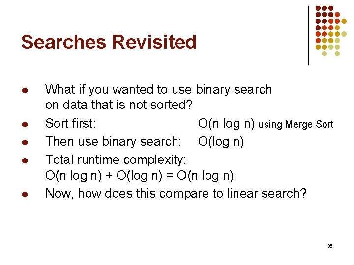
Searches Revisited l l l What if you wanted to use binary search on data that is not sorted? Sort first: O(n log n) using Merge Sort Then use binary search: O(log n) Total runtime complexity: O(n log n) + O(log n) = O(n log n) Now, how does this compare to linear search? 36

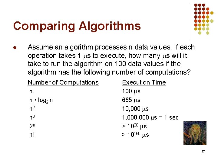
Comparing Algorithms l Assume an algorithm processes n data values. If each operation takes 1 s to execute, how many s will it take to run the algorithm on 100 data values if the algorithm has the following number of computations? Number of Computations n n • log 2 n n 2 n 3 2 n n! Execution Time 100 s 665 s 10, 000 s 1, 000 s = 1 sec > 1030 s > 10160 s 37