Algorithms in Action Fast Fourier Transform Haim Kaplan

Algorithms in Action Fast Fourier Transform Haim Kaplan, Uri Zwick Tel Aviv University March 2016 Last updated: March 16, 2016 1

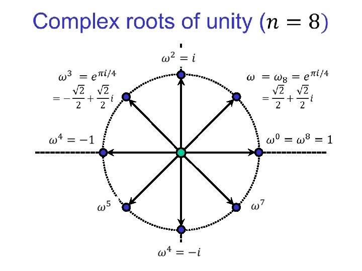
Discrete Fourier Transform (DFT) A very special linear transformation 2

Discrete Fourier Transform (DFT) 4

DFT as polynomial evaluation

Fast Fourier Transform (FFT) FFT is an algorithm for computing DFT. Developed by Cooley and Tuckey in 1965, but similar ideas were used much earlier, e. g. , by Runge and König in 1924 and others. 6

Applications of the FFT Digital signal processing: Transforming signals from time to frequency domain Computing convolutions: Multiplication of polynomials Multiplication of large integers String matching problems Quantum computing: Used in Shor’s integer factorization algorithm

Sampling rate = 32 Hz 8

Sampling rate = 32 Hz 9

Spectrum = absolute value of the Fourier coefficients. In addition to the spectrum, we also have the phase. 9 (=9 Hz) is right. What is 23?

Same samples at 16 Hz. 11

The Sampling Theorem (Nyquist, Shannon, …) For information only. Not part of this course. We only consider finite discrete “signals”. 12

“Symmetry” of DFT for real signals Exercise: Prove the lemma. For real inputs, the first half of the DFT contains all the information. 13

Frequencies and their relative contribution correctly identified! As we shall soon see, from the Fourier coefficients, not just their absolute values, we can reconstruct the original signal. 14

Basis vectors correspond to integer frequencies. 9. 5 Hz is a non-trivial combination of basis vectors. See below. 15

For more information, take a course on digital signal processing. 16

Decomposing the DFT (I) 17

Decomposing the DFT (II) 18

FFT – recursive version 19

20

Complexity of the FFT

A butterfly “Twiddle factor” + 22

Input permuted! An FFT circuit

An FFT circuit Input further permuted!

Input permuted! An FFT circuit

Bit-reversal permutation An FFT circuit

Bit-reversal permutation An FFT circuit

FFT and Algorithm Engineering In real life, constant factors matter. A tremendous amount of work was invested is optimizing the performance of FFT algorithms on specific architectures. The algorithm we saw is a radix-2 FFT. Radix-4 and varying radices work better in practice. A good FFT implementation should use cache and memory cleverly, and use parallelism if possible. 28

The Inverse DFT The inverse DFT is very similar to the DFT: To prove it, we need show that

The Inverse DFT 30

Change of basis 32

Orthonormal basis Conjugate transpose 33

Orthonormal basis 34

The Fourier basis is orthonormal.

Why did the “signal processing” examples work? Note: The values shown on slide 14 are normalized absolute values. 36

A butterfly and its inverse + 37

Convolution

Convolution For convenience

Convolution Compute products for each aligment. 40

Convolution 41

Convolution and polynomial multiplication 42

Cyclic Convolution

Convolution Cyclic Convolutions can be reduced to cyclic convolutions by padding. 44

The Convolution Theorem Cyclic convolution Point-wise multiplication Proof idea:

Proof of Convolution Theorem The claim follows as the interpolation polynomial is unique. Uniqueness follows from the fact that DFT is invertible.

The Chirp Transform

Polynomial arithmetic

Karatsuba’s algorithm

Numerical issues So far, we assumed that all arithmetical operations are exact. The FFT algorithm is well-behaved numerically. The errors introduced if all operations are done using floating-point arithmetic are relatively small. In signal processing applications small errors are acceptable. 50

Integer Polynomial Multiplication We now want to add and multiply polynomials with integer coefficients. We want an exact result. (Proof omitted. )

Integer Multiplication There are practical applications, e. g. , cryptography, that require multiplying very large integers. Can we use FFTs to obtain a aster integer multiplication algorithm/circuit? Yes, as integer multiplication can be reduced to polynomial multiplication. 52

Schönhage-Strassen’s algorithm Basic idea Some clever tricks are used to speed-up the algorithm.

Schönhage-Strassen’s algorithm

Schönhage-Strassen’s algorithm Adding these 3 integers gives us the final answer. 55

Schönhage-Strassen’s algorithm The final step 56

Schönhage-Strassen’s algorithm Number of bit operations per each arithmetical operation.

Schönhage-Strassen’s algorithm

Integer Multiplication [Schönhage-Strassen (1971)] obtained an improved version of their algorithm with a running time of ? ? ? No numerical issues! [Fürer (2007)] and [De-Kurur-Saha-Saptharishi (2008)] improved the running time to 59

DFT and FFT in rings

Rings 61

Rings and Fields 62

Modular arithmetic

Generators of prime fields

FFT in prime fields Example: Multiply two integer polynomials of degree < 512. But, we will get the coefficients modulo 12, 289 …

FFT in prime fields Example: Multiply two integer polynomials of degree < 512. Modular arithmetic may be more “elegant”. We don’t have to worry about numerical errors. But, modular arithmetic is not necessarily faster than working with floating point complex numbers. We need to find appropriate prime numbers and generators. 66

FFT using modular arithmetic To support DFT and FFT a ring does not have to be a field. The main advantage of using modular arithmetic comes from choosing rings with very special primitive roots of unity.

Schönhage-Strassen’s algorithm

String Matching abracadabraabara abracadabra 69

More String Matching Problems abracadabraabara abracadabra Count the number of matches/mismatches in each alignment of the pattern with the text. “Traditional” string matching techniques are not so efficient for these extensions. 70

(Cross-)Correlation 71

(Cross-)Correlation A convolution without the initial reversal, with a shift of indices.

Counting mismatches [Fischer-Paterson (1974)]

Counting mismatches with wildcards [Fischer-Paterson (1974)] 74

75

76

Exact matches with wildcards [Clifford-Clifford (2007)] Replace each character by a positive integer. Replace the wildcard by 0. 77

Exact matches with wildcards [Clifford-Clifford (2007)]

Bonus material Not covered in class this term “Careful. We don’t want to learn from this. ” (Calvin in Bill Watterson’s “Calvin and Hobbes”) 79

Continuous Fourier Transform (Some conditions apply. ) 80

Fourier series where: (Some conditions apply. ) 81

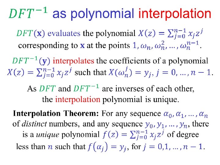
Polynomial interpolation which can be found by solving the linear equations: A solution exists and is unique because the matrix, known as a Vandermonde matrix, is non-singular.

Vandermonde Determinant

Lagrange formula can be obtained as follows: 84

Output the numbers in the matrix column by column. 85

86

87

Negative Cyclic Convolution: Negative Cyclic Convolution:

Negative Cyclic Convolution A naïve way of computing the negative cyclic convolution is to first compute the non-cyclic convolution. This saves a factor of 2 and plays an important role in the modular Schönhage-Strassen algorithm.

Modular Schönhage-Strassen

Modular Schönhage-Strassen

Modular Schönhage-Strassen 93