Algorithms for solving sequential zerosum completeinformation games Tuomas

Algorithms for solving sequential (zero-sum) complete-information games Tuomas Sandholm

CHESS, MINIMAX SEARCH, AND IMPROVEMENTS TO MINIMAX SEARCH

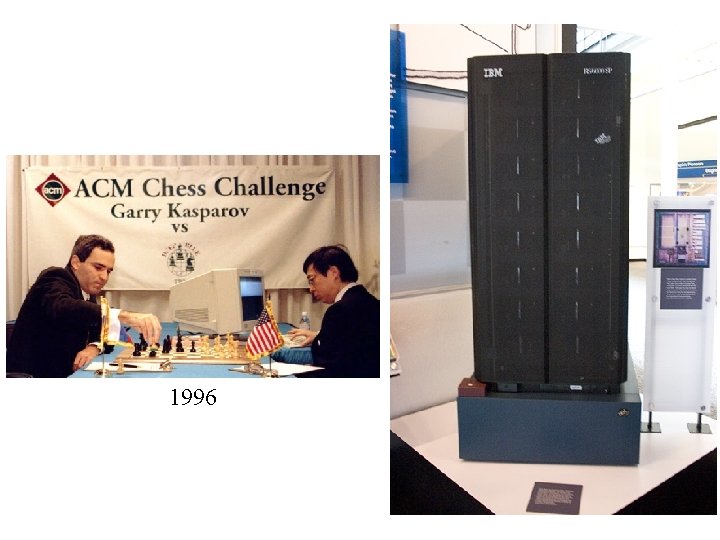
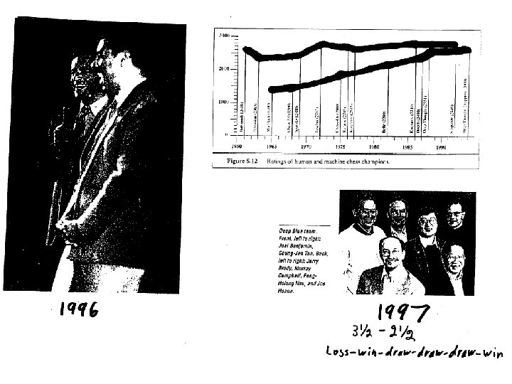
1996

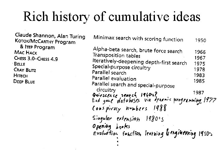
Rich history of cumulative ideas

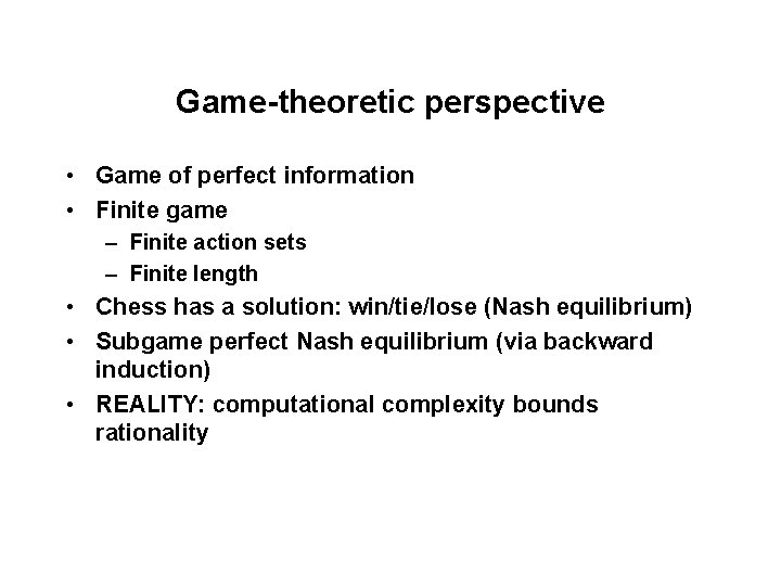
Game-theoretic perspective • Game of perfect information • Finite game – Finite action sets – Finite length • Chess has a solution: win/tie/lose (Nash equilibrium) • Subgame perfect Nash equilibrium (via backward induction) • REALITY: computational complexity bounds rationality

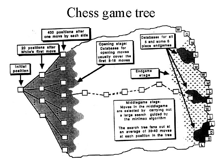
Chess game tree

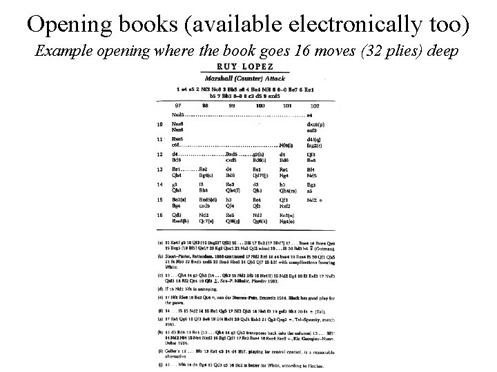
Opening books (available electronically too) Example opening where the book goes 16 moves (32 plies) deep

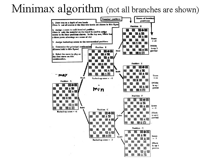
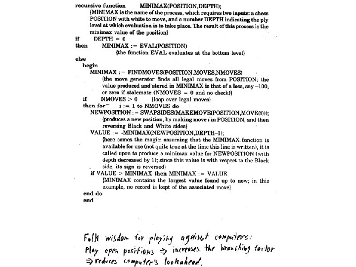
Minimax algorithm (not all branches are shown)

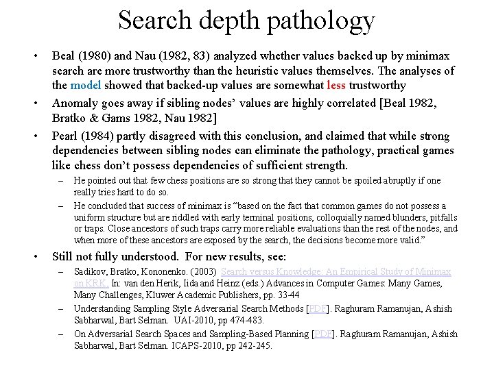
Search depth pathology • • • Beal (1980) and Nau (1982, 83) analyzed whether values backed up by minimax search are more trustworthy than the heuristic values themselves. The analyses of the model showed that backed-up values are somewhat less trustworthy Anomaly goes away if sibling nodes’ values are highly correlated [Beal 1982, Bratko & Gams 1982, Nau 1982] Pearl (1984) partly disagreed with this conclusion, and claimed that while strong dependencies between sibling nodes can eliminate the pathology, practical games like chess don’t possess dependencies of sufficient strength. – – • He pointed out that few chess positions are so strong that they cannot be spoiled abruptly if one really tries hard to do so. He concluded that success of minimax is “based on the fact that common games do not possess a uniform structure but are riddled with early terminal positions, colloquially named blunders, pitfalls or traps. Close ancestors of such traps carry more reliable evaluations than the rest of the nodes, and when more of these ancestors are exposed by the search, the decisions become more valid. ” Still not fully understood. For new results, see: – – – Sadikov, Bratko, Kononenko. (2003) Search versus Knowledge: An Empirical Study of Minimax on KRK, In: van den Herik, Iida and Heinz (eds. ) Advances in Computer Games: Many Games, Many Challenges, Kluwer Academic Publishers, pp. 33 -44 Understanding Sampling Style Adversarial Search Methods [PDF]. Raghuram Ramanujan, Ashish Sabharwal, Bart Selman. UAI-2010, pp 474 -483. On Adversarial Search Spaces and Sampling-Based Planning [PDF]. Raghuram Ramanujan, Ashish Sabharwal, Bart Selman. ICAPS-2010, pp 242 -245.

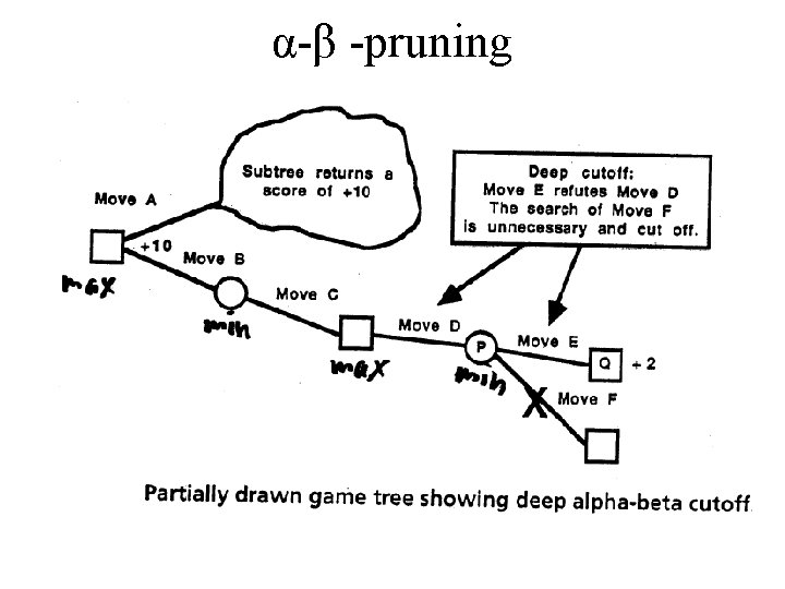
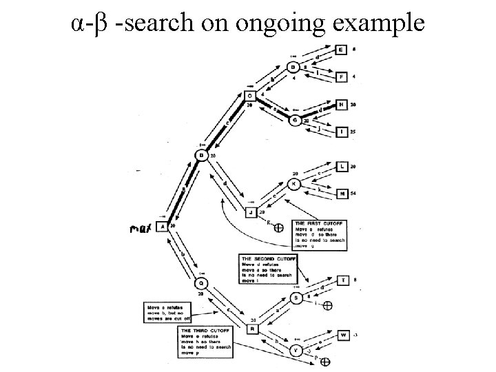
α-β -pruning

α-β -search on ongoing example

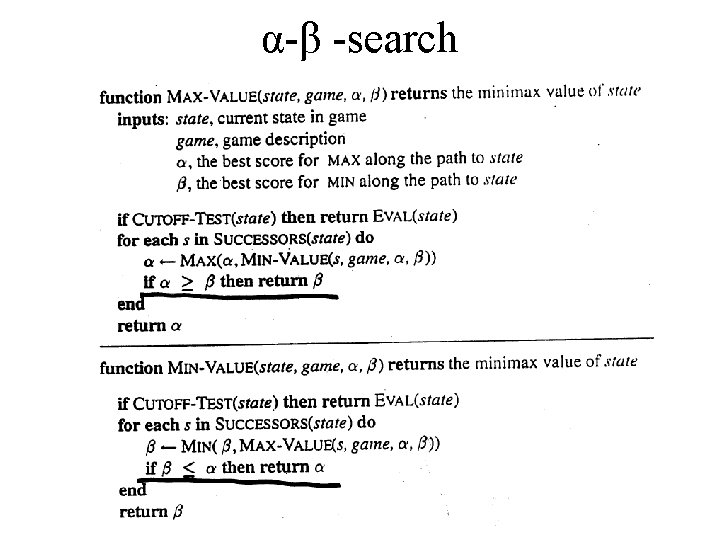
α-β -search

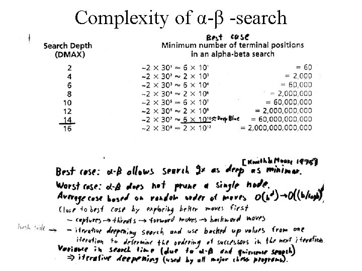
Complexity of α-β -search

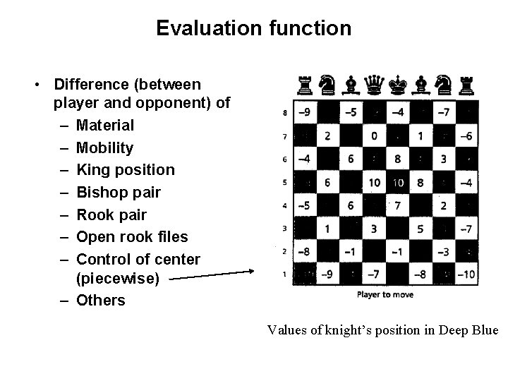
Evaluation function • Difference (between player and opponent) of – Material – Mobility – King position – Bishop pair – Rook pair – Open rook files – Control of center (piecewise) – Others Values of knight’s position in Deep Blue

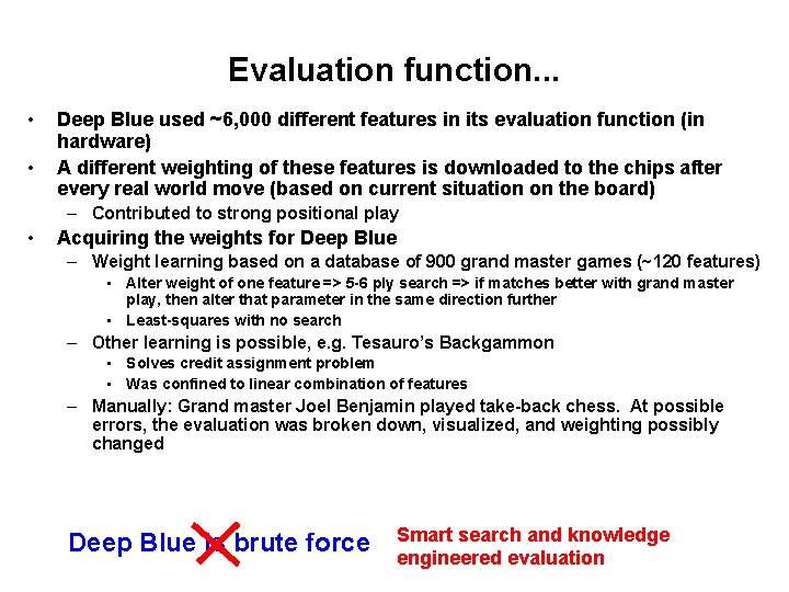
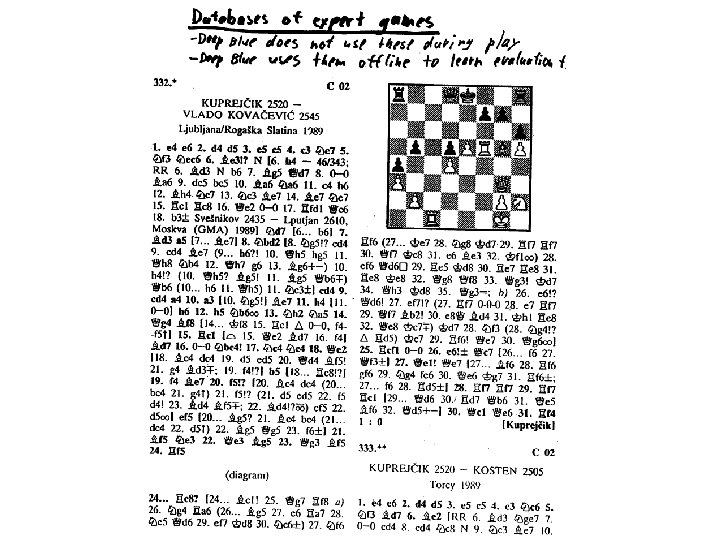
Evaluation function. . . • • Deep Blue used ~6, 000 different features in its evaluation function (in hardware) A different weighting of these features is downloaded to the chips after every real world move (based on current situation on the board) – Contributed to strong positional play • Acquiring the weights for Deep Blue – Weight learning based on a database of 900 grand master games (~120 features) • Alter weight of one feature => 5 -6 ply search => if matches better with grand master play, then alter that parameter in the same direction further • Least-squares with no search – Other learning is possible, e. g. Tesauro’s Backgammon • Solves credit assignment problem • Was confined to linear combination of features – Manually: Grand master Joel Benjamin played take-back chess. At possible errors, the evaluation was broken down, visualized, and weighting possibly changed Deep Blue is brute force Smart search and knowledge engineered evaluation

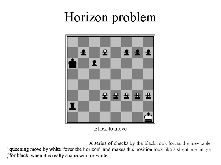
Horizon problem

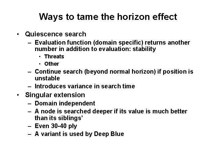
Ways to tame the horizon effect • Quiescence search – Evaluation function (domain specific) returns another number in addition to evaluation: stability • Threats • Other – Continue search (beyond normal horizon) if position is unstable – Introduces variance in search time • Singular extension – Domain independent – A node is searched deeper if its value is much better than its siblings’ – Even 30 -40 ply – A variant is used by Deep Blue

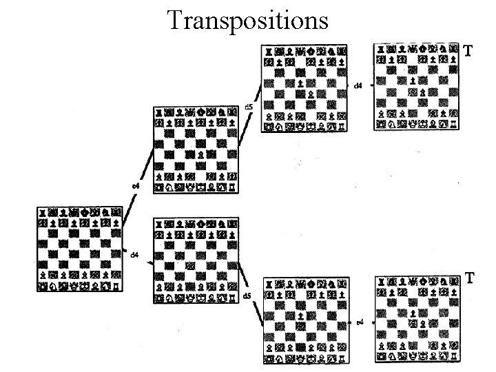
Transpositions

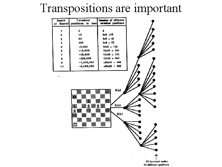
Transpositions are important

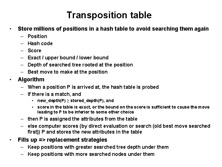
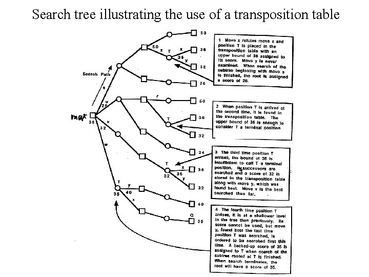
Transposition table • Store millions of positions in a hash table to avoid searching them again – – – • Position Hash code Score Exact / upper bound / lower bound Depth of searched tree rooted at the position Best move to make at the position Algorithm – When a position P is arrived at, the hash table is probed – If there is a match, and • new_depth(P) ≥ stored_depth(P), and • score in the table is exact, or the bound on the score is sufficient to cause the move leading to P to be inferior to some other choice – then P is assigned the attributes from the table – else computer scores (by direct evaluation or search (old best move searched first)) P and stores the new attributes in the table • Fills up => replacement strategies – Keep positions with greater searched tree depth under them – Keep positions with more searched nodes under them

Search tree illustrating the use of a transposition table

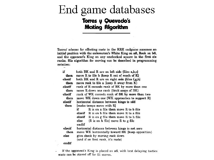
End game databases

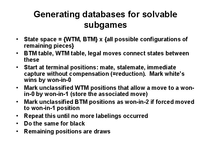
Generating databases for solvable subgames • State space = {WTM, BTM} x {all possible configurations of remaining pieces} • BTM table, WTM table, legal moves connect states between these • Start at terminal positions: mate, stalemate, immediate capture without compensation (=reduction). Mark white’s wins by won-in-0 • Mark unclassified WTM positions that allow a move to a wonin-0 by won-in-1 (store the associated move) • Mark unclassified BTM positions as won-in-2 if forced moved to won-in-1 position • Repeat this until no more labelings occurred • Do the same for black • Remaining positions are draws

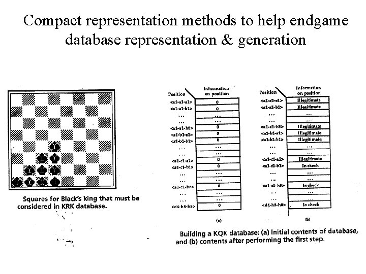
Compact representation methods to help endgame database representation & generation

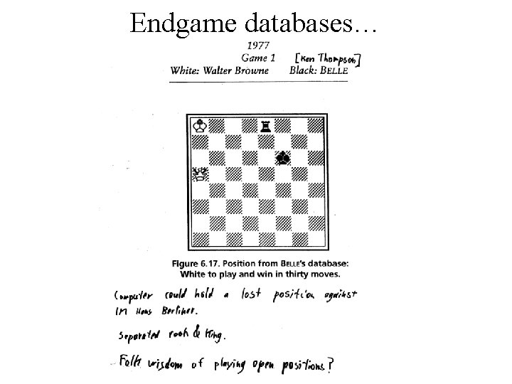
Endgame databases…

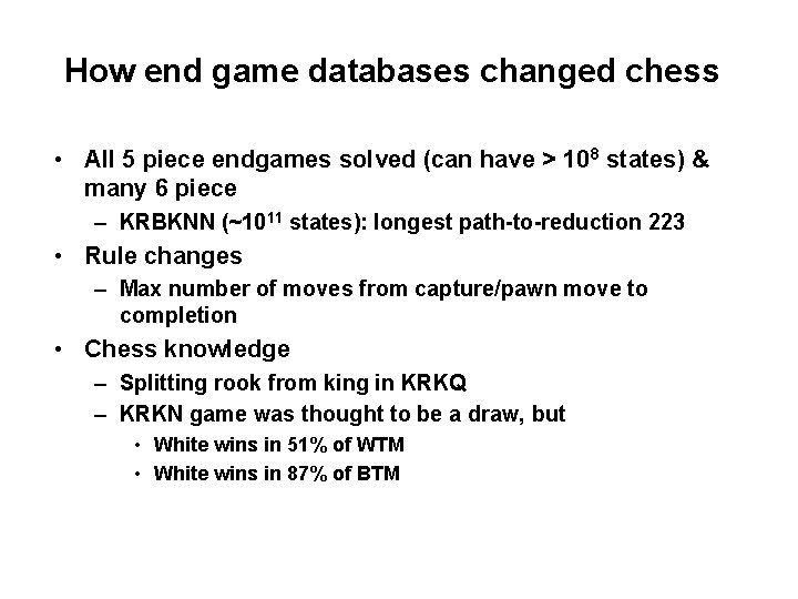
How end game databases changed chess • All 5 piece endgames solved (can have > 108 states) & many 6 piece – KRBKNN (~1011 states): longest path-to-reduction 223 • Rule changes – Max number of moves from capture/pawn move to completion • Chess knowledge – Splitting rook from king in KRKQ – KRKN game was thought to be a draw, but • White wins in 51% of WTM • White wins in 87% of BTM

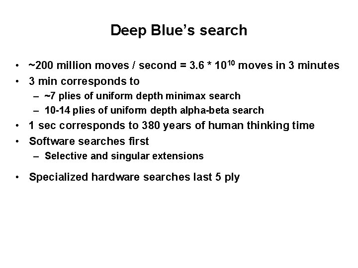
Deep Blue’s search • ~200 million moves / second = 3. 6 * 1010 moves in 3 minutes • 3 min corresponds to – ~7 plies of uniform depth minimax search – 10 -14 plies of uniform depth alpha-beta search • 1 sec corresponds to 380 years of human thinking time • Software searches first – Selective and singular extensions • Specialized hardware searches last 5 ply

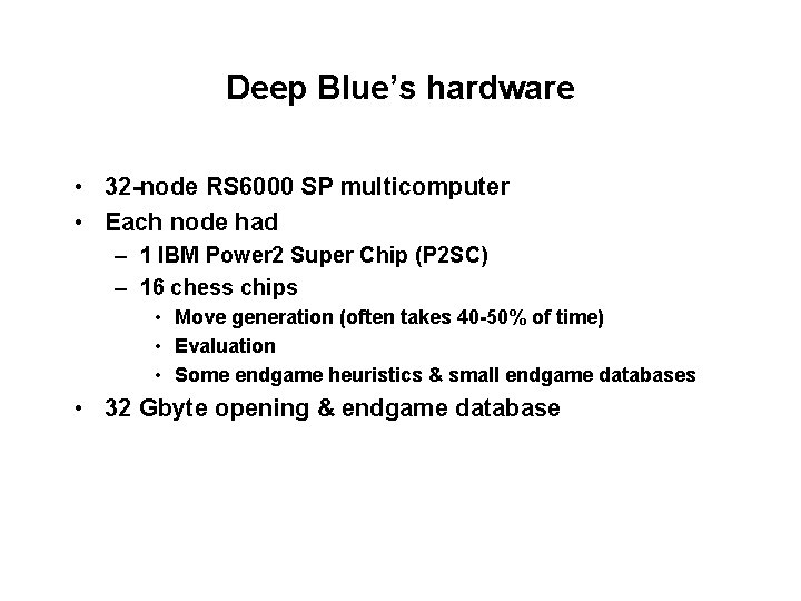
Deep Blue’s hardware • 32 -node RS 6000 SP multicomputer • Each node had – 1 IBM Power 2 Super Chip (P 2 SC) – 16 chess chips • Move generation (often takes 40 -50% of time) • Evaluation • Some endgame heuristics & small endgame databases • 32 Gbyte opening & endgame database

Role of computing power

Interestingly…Freestyle Chess • Hybrid human-AI chess players are stronger than humans or AI alone

GO, MONTE CARLO TREE SEARCH, AND COMBINING IT WITH DEEP LEARNING

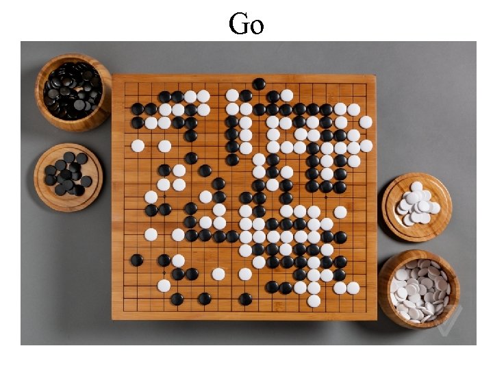
Go

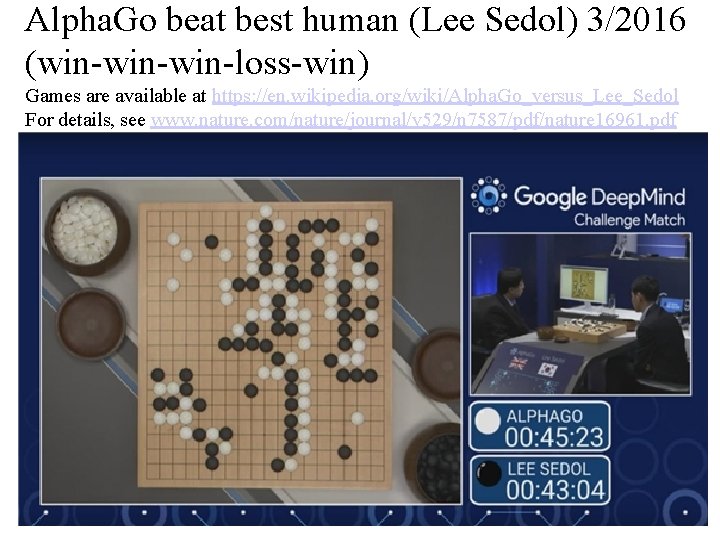
Alpha. Go beat best human (Lee Sedol) 3/2016 (win-win-loss-win) Games are available at https: //en. wikipedia. org/wiki/Alpha. Go_versus_Lee_Sedol For details, see www. nature. com/nature/journal/v 529/n 7587/pdf/nature 16961. pdf

Alpha. Go Zero beat Alpha. Go 100 -0 in Oct 2017 www. nature. com/articles/nature 24270. pdf • Alpha. Go started with supervised learning based on human expert games, and then used reinforcement learning to tune the neural networks • Alpha. Go Zero used no supervised learning, just reinforcement learning to tune the neural networks

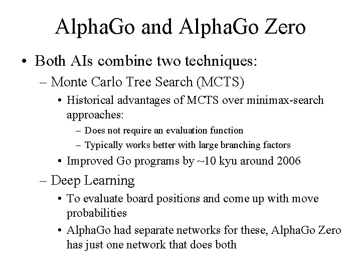
Alpha. Go and Alpha. Go Zero • Both AIs combine two techniques: – Monte Carlo Tree Search (MCTS) • Historical advantages of MCTS over minimax-search approaches: – Does not require an evaluation function – Typically works better with large branching factors • Improved Go programs by ~10 kyu around 2006 – Deep Learning • To evaluate board positions and come up with move probabilities • Alpha. Go had separate networks for these, Alpha. Go Zero has just one network that does both

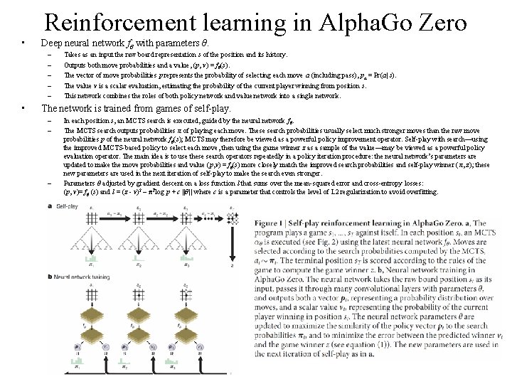
Reinforcement learning in Alpha. Go Zero • Deep neural network fθ with parameters θ. – – – • Takes as an input the raw board representation s of the position and its history. Outputs both move probabilities and a value, (p, v) = fθ(s). The vector of move probabilities p represents the probability of selecting each move a (including pass), pa = Pr(a| s). The value v is a scalar evaluation, estimating the probability of the current player winning from position s. This network combines the roles of both policy network and value network into a single network. The network is trained from games of self-play. – – – In each position s, an MCTS search is executed, guided by the neural network fθ. The MCTS search outputs probabilities π of playing each move. These search probabilities usually select much stronger moves than the raw move probabilities p of the neural network fθ(s); MCTS may therefore be viewed as a powerful policy improvement operator. Self-play with search—using the improved MCTS-based policy to select each move, then using the game winner z as a sample of the value—may be viewed as a powerful policy evaluation operator. The main idea is to use these search operators repeatedly in a policy iteration procedure: the neural network’s parameters are updated to make the move probabilities and value (p, v) = fθ(s) more closely match the improved search probabilities and self-play winner ( π, z); these new parameters are used in the next iteration of self-play to make the search even stronger. Parameters θ adjusted by gradient descent on a loss function l that sums over the mean-squared error and cross-entropy losses: (p, v)= fθ (s) and l = (z - v)2 – πTlog p + c ||θ|| where c is a parameter that controls the level of L 2 regularization to avoid overfitting.

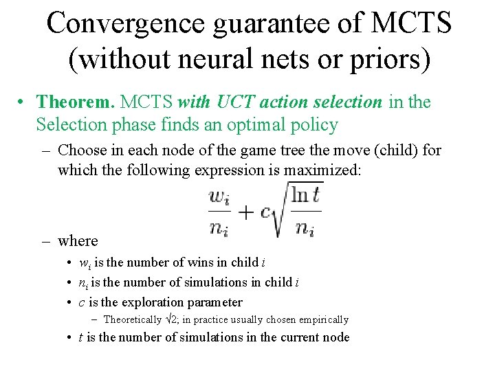
Convergence guarantee of MCTS (without neural nets or priors) • Theorem. MCTS with UCT action selection in the Selection phase finds an optimal policy – Choose in each node of the game tree the move (child) for which the following expression is maximized: – where • wi is the number of wins in child i • ni is the number of simulations in child i • c is the exploration parameter – Theoretically √ 2; in practice usually chosen empirically • t is the number of simulations in the current node

Alpha. Go Zero • One machine that had 4 Tensor Processing Units (TPUs) • First version had 72 hours of training, second version had 40 days